Conservation of preparatory neural events in monkey motor cortex regardless of how movement is initiated
- Columbia University Medical Center, United States
- Columbia University, United States
- Columbia University Medical Center, Unitedstate
Figures
Figure 1
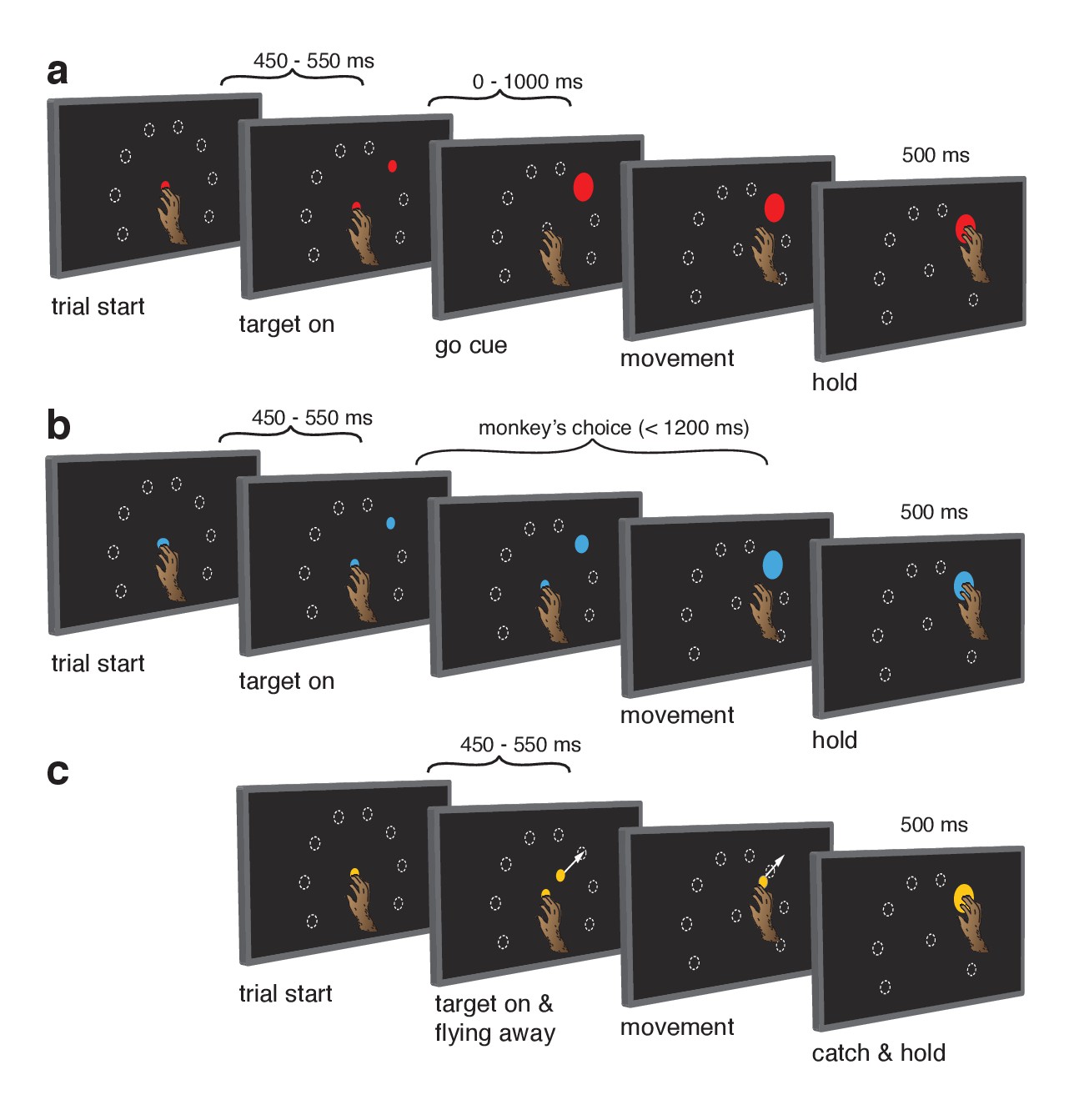
Behavioral task.
Monkeys performed the same set of reaches under three initiation contexts. (a) Cue-initiated context. Each trial began when the monkey touched a red central point on the screen. After a brief hold period (450–550 ms) a red target appeared in one of eight possible locations (white dashed circles, not visible to the monkey) 130 mm from the touch point. After a variable delay period (0–1000 ms) the target suddenly increased in size providing the go cue to initiate the reach. (b) Self-initiated context. Trials began as above, but the central point was blue. Subsequently, a small blue target appeared and gradually grew in size. Monkeys were free to initiate the reach as soon as the target appeared on the screen. However longer waiting times were rewarded with juice rewards. (c) Quasi-automatic context. The central point was yellow. Yellow targets appeared in one of eight possible locations. The initial target location was 40 mm from the touch point. Immediately after appearing, the target moved radially outward. Monkeys had to intercept the target before it reached the edge of the screen and disappeared. Given typical reaction times, target interception occurred at a location near the location of the targets in the other two tasks (dashed circles).
Figure 2 with 2 supplements
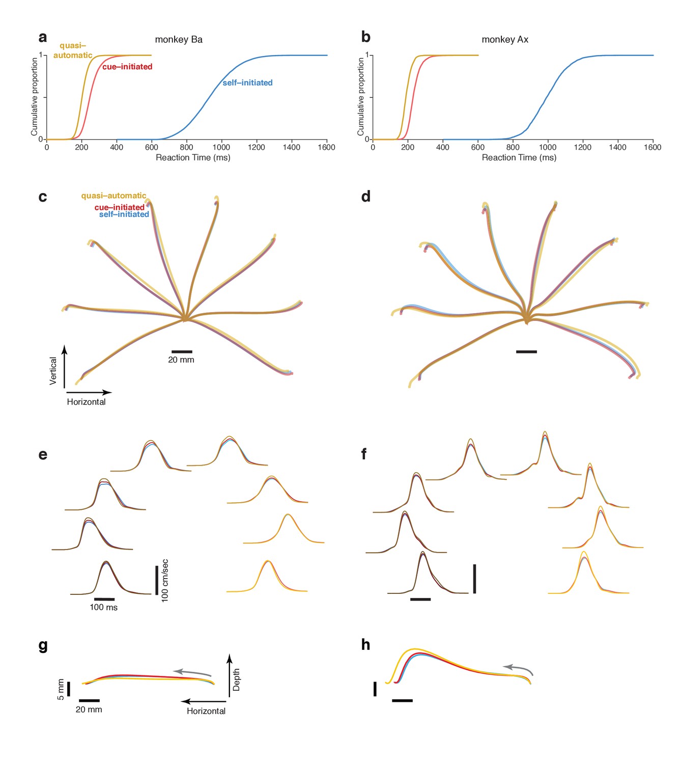
Reaction time distributions and reach kinematics.
(a,b) cumulative reaction time distributions for the three contexts. Trials are pooled across all recordings. Data for monkey Ba and Ax are shown in the left and right columns respectively. (c,d) Average reach trajectories for the eight targets and three contexts. (e,f) Average speed profiles in the three contexts, using the same color coding as above. Line shade indicates reach direction: light traces for rightwards reaches and dark traces for leftwards reaches. This same shade-coding is preserved in subsequent figures. (g,h) Average reach trajectories for one example reach direction (leftward) with depth shown on an expanded scale to allow closer examination of trajectories in that dimension. Gray arrows indicate direction in which the hand traveled.
Figure 2—figure supplement 1
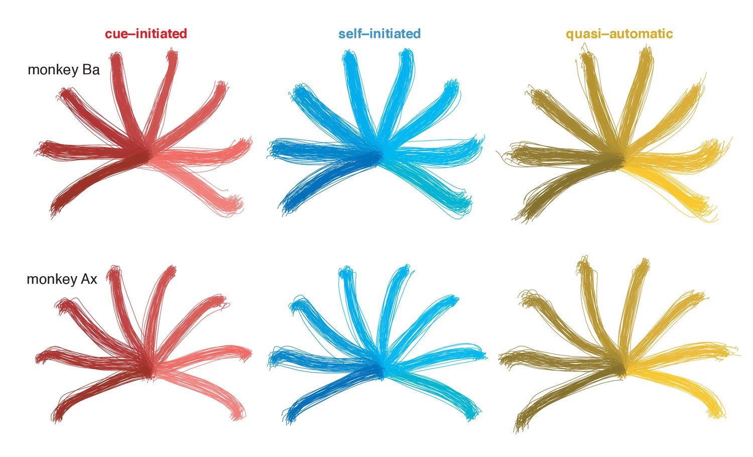
Individual-trial reach trajectories from a typical session.
Reach trajectories are fairly stereotyped across trials and were similar for the three contexts.
Figure 2—figure supplement 2
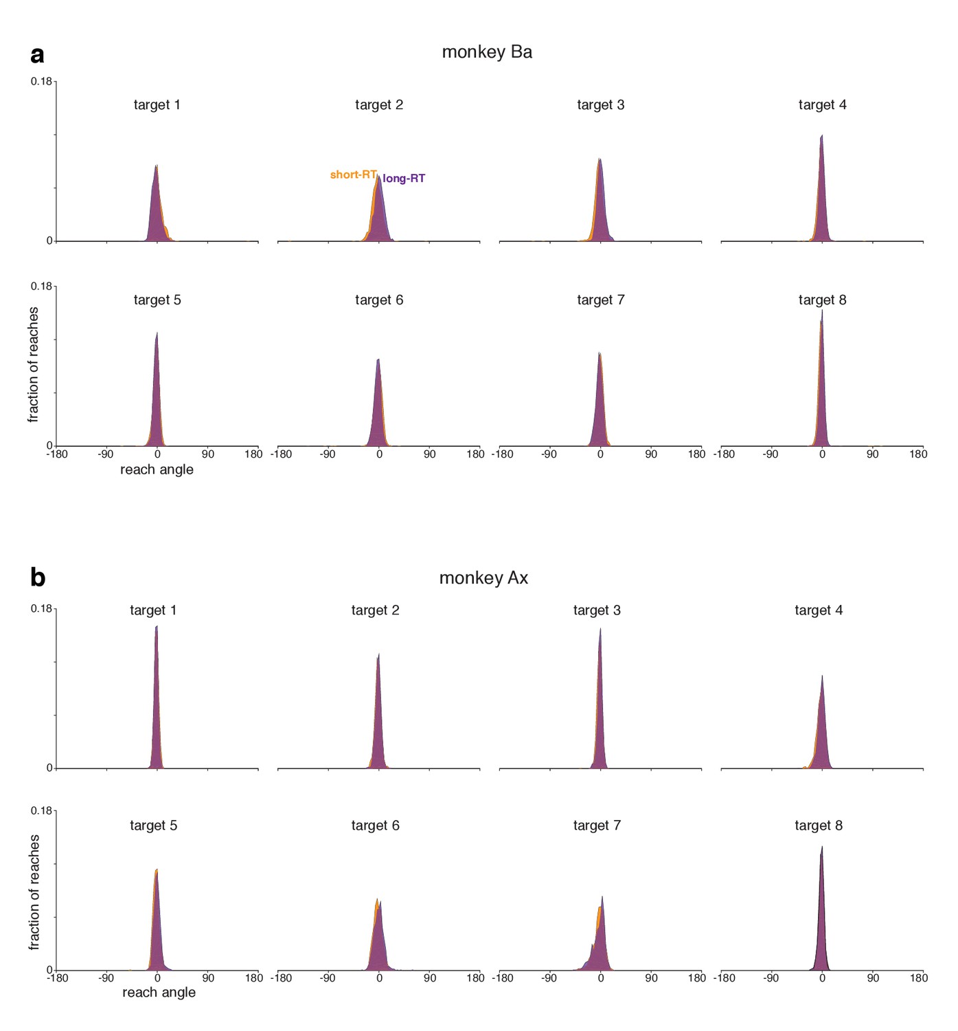
Distributions of initial reach angle during the quasi-automatic context.
(a) Data for monkey Ba. Reach angle was measured 100 ms after reach onset. Distributions include both successful trials and trials where a reach was executed but missed the target. Distributions include trials for all recording sessions. Data are shown separately for all target locations. Reach angle was measured relative to target angle, so that 0 degrees indicates a reach directed exactly at the target. Separate distributions are plotted for trials with RTs shorter than the median (orange) versus longer than the median (purple). In both cases, the initial reach angle was close to the target direction on essentially all trials. In particular there is no evidence of guessing, or of randomly chosen directions, for the shorter RTs. (b) Data for monkey Ax.
Figure 3 with 1 supplement
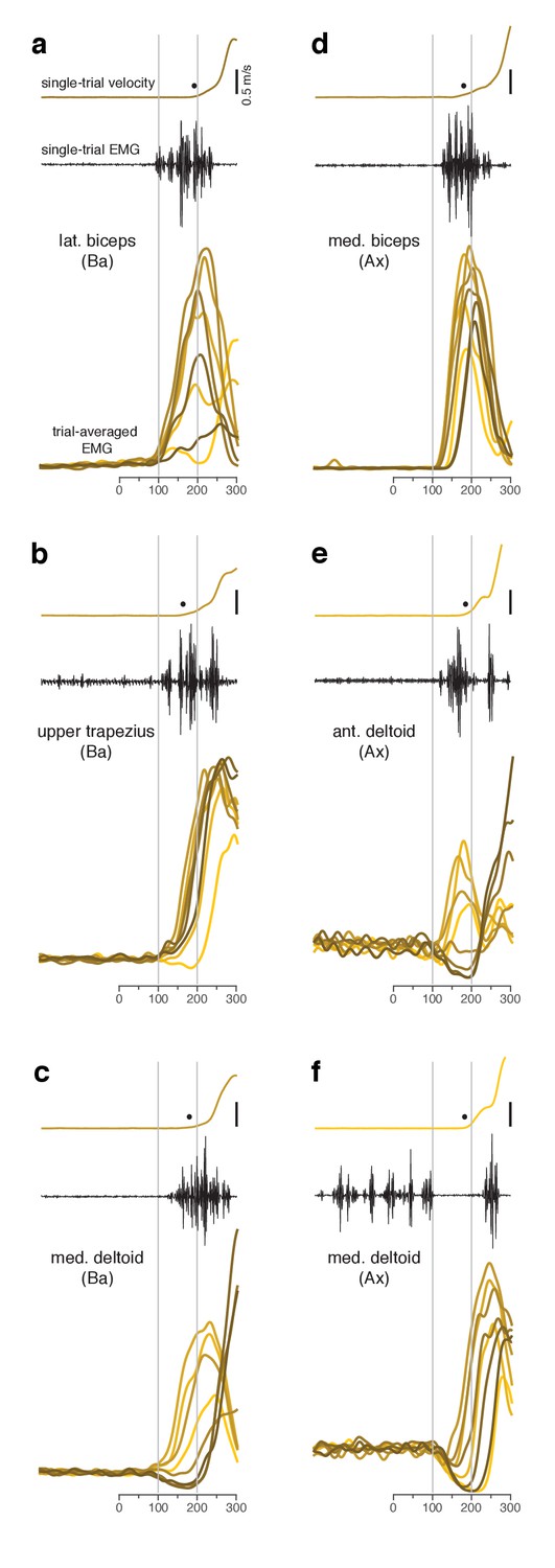
Muscle activity analyzed relative to target onset during the quasi-automatic context.
(a–f) Each panel plots data for one muscle.Single-trial examples of hand velocity (yellow) and EMG (black) are shown at the top of each panel. Filled circle indicates the estimated time of movement onset on that trial. Average rectified-and-filtered EMG is shown, for each target direction, at the bottom of each panel. Averages were made locked to target onset. Thus, the first change provides an estimate of how soon EMG could change on trials with faster RTs. Filtering used a 10 ms Gaussian to minimize impact on latency. Shade-coding indicates reach direction as in Figure 2. Gray vertical lines mark 100 ms and 200 ms after target onset. Note that the target-locked averages used here do not use concatenation and are most appropriate for examining latency. Subsequent analyses employ concatenated averages, with movement-related activity locked to movement onset, which is more appropriate when examining activity patterns.
Figure 3—figure supplement 1
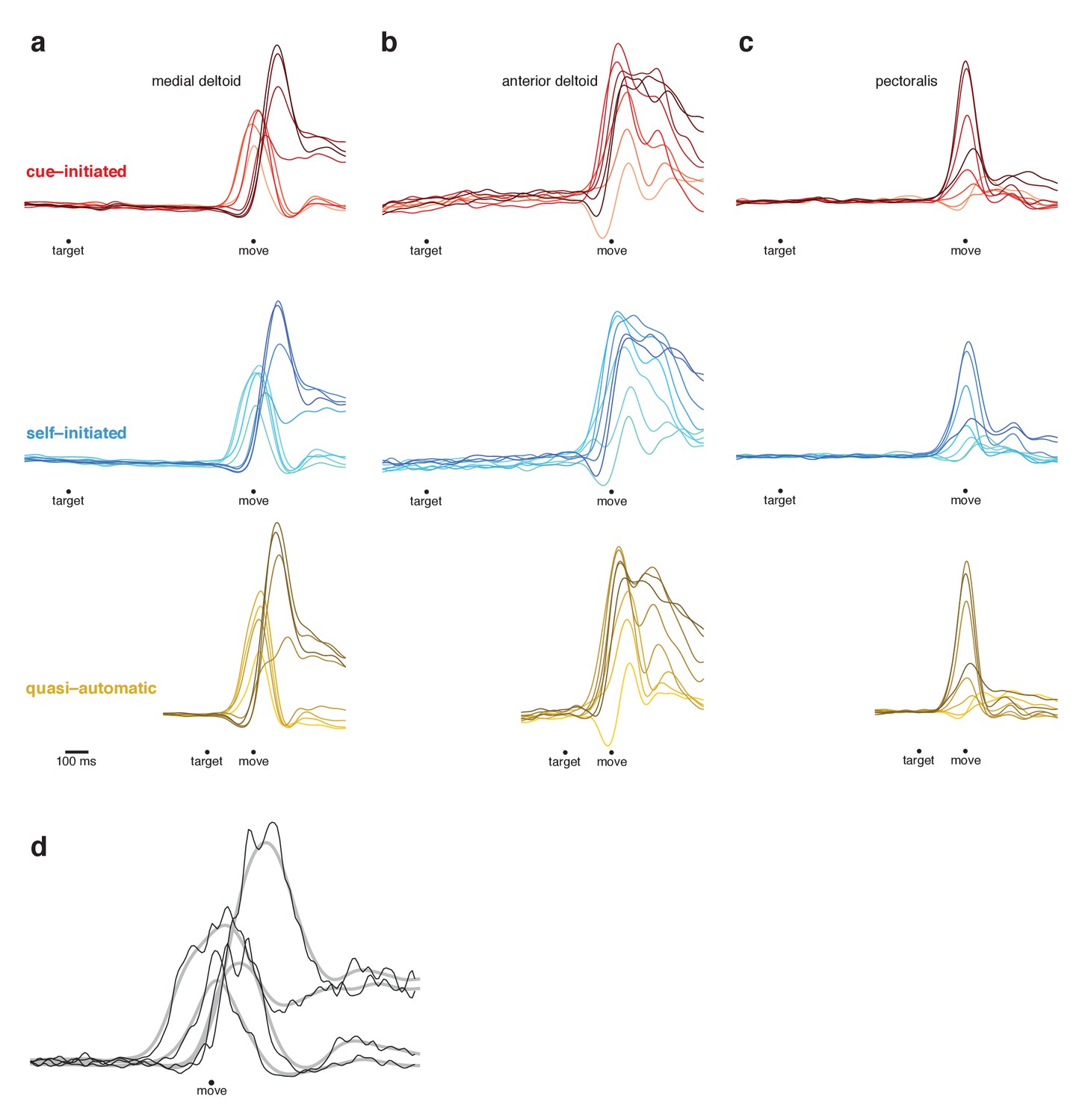
Responses from three muscles of the upper arm.
(a–c) Comparison of muscle activity across contexts (rows). Each column plots the response of one muscle, recorded from monkey Ba. Each trace plots the response for one reach direction. Individual EMG records were rectified before smoothing with a 20 ms Gaussian and averaging. Averaging was performed on concatenated target-locked and movement-locked data, as for the neural responses. Averages were computed across many trials (up to 60 trials/condition) and are therefore quite smooth and noise-free. (d) Illustration of the impact of different filters. EMG for the medial deltoid, shown on an expanded scale for four reach directions. Black traces show average EMG with very minimal filtering (a 5 ms Gaussian) and gray traces show average EMG with standard filtering (20 ms Gaussian). The 20 ms filter slightly reduces amplitude and has a minor impact on latency. Responses are otherwise similar regardless of filtering but are, as expected, noisier when using the 5 ms Gaussian. Based on these tradeoffs, we chose a 20 ms filter for most analyses and a 10 ms filter for analyses of latency.
Figure 4 with 2 supplements

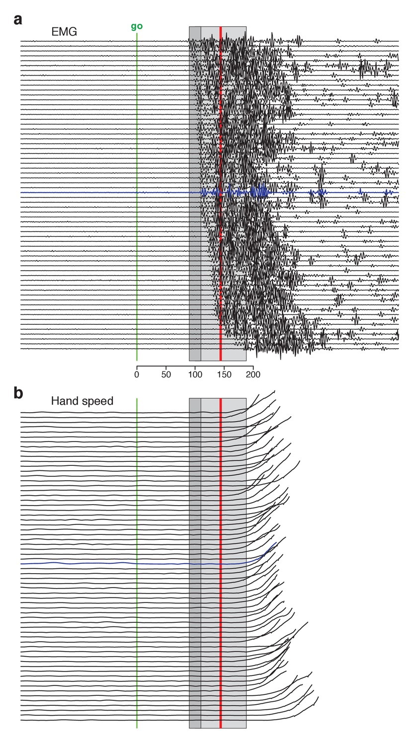
Single-trial EMG voltages during the quasi-automatic context, ordered by response latency.
EMG data were recorded from the trapezius of monkey Ba. This recording (different from that in Figure 3b) had low baseline activity, making it possible to estimate EMG onset on individual trials. (a) Each trace plots the voltage recorded on a single trial. Ordering is based on estimated EMG onset latency. Blue trace indicates the trial with the median latency. EMG onset was estimated via inspection; trials were not analyzed if baseline EMG was not essentially zero. This was critical because fluctuations in a non-zero baseline produced ambiguity when assessing EMG onset. Analysis included trials for three reach directions that evoked the largest response. Shaded regions allow comparison with EMG latencies in Perfiliev et al. (2010). For that study, the earliest EMG was observed at 90–110 ms (range is across subjects) and the mean onset of EMG was 144 (averaged across trials and subjects). These benchmarks are indicated by the dark gray shaded region and the red line respectively. The estimated typical within-subject range of latencies for Perfiliev is indicated by the light gray shaded region. This was estimated as symmetric about the across-subject mean, beginning at the average earliest latency (thus spanning from 44 ms below to 44 ms above the mean). (b) Hand-speed traces for the same trials as in panel a, using the same ordering. Traces are truncated to allow magnification of early events.
Figure 4—figure supplement 1
Same as Figure 4 but for the biceps of monkey Ba.
Trials are combined across two recordings from the biceps, and across the three target directions that evoked the largest response.
Figure 4—figure supplement 2
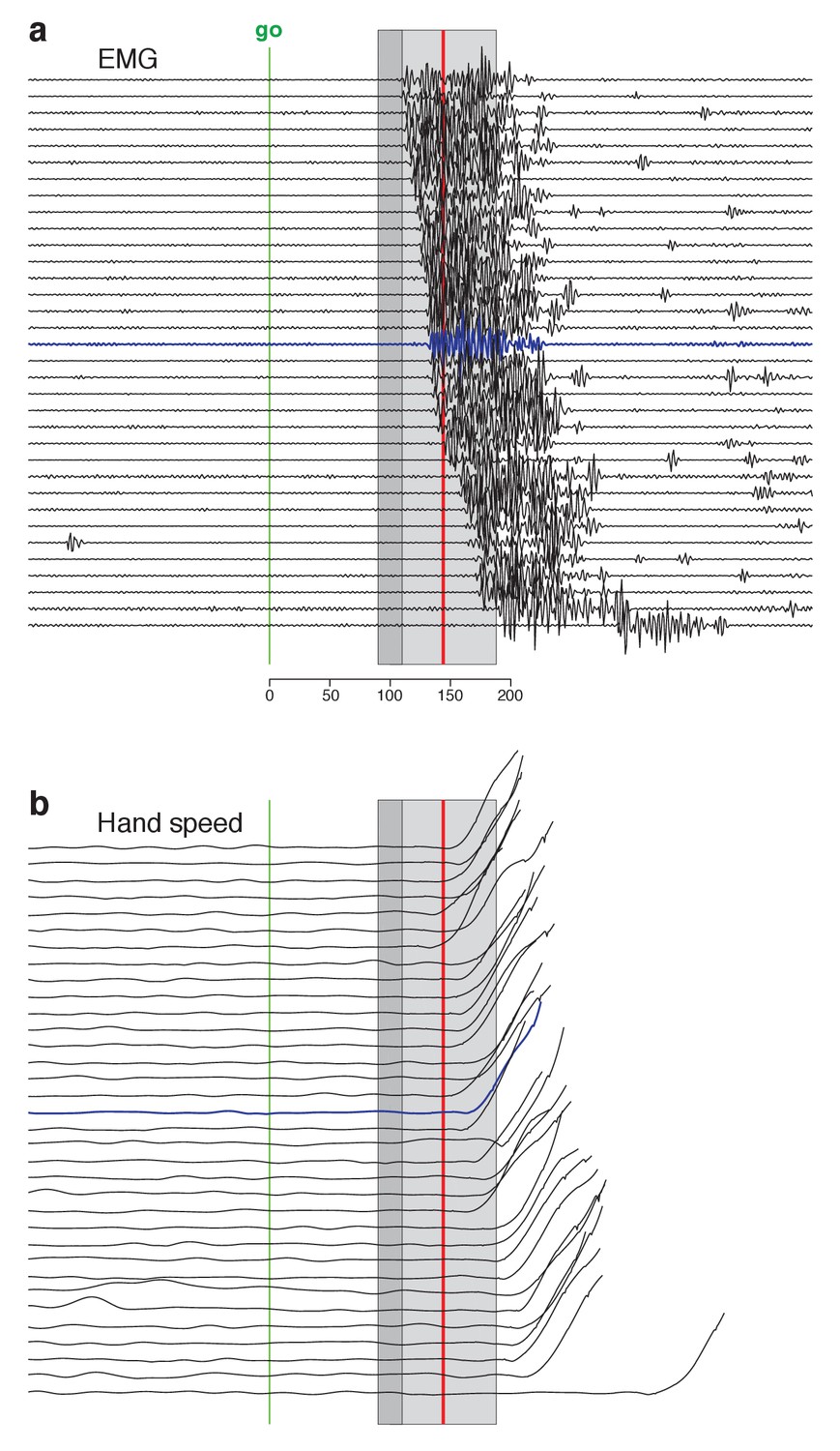
Same as Figure 4 but for the biceps of monkey Ax.
Trials are combined across the three target directions that evoked the largest response.
Figure 5
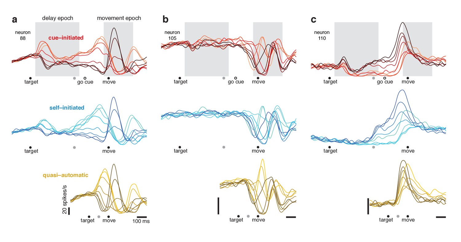
Responses of three example neurons.
Each column shows the responses of a single neuron for the three contexts. Each trace plots the trial-averaged firing rate for one reach direction (same color scheme as in Figure 2). Gray shaded regions indicate delay and movement epochs, used to define the preparatory and movement dimensions in subsequent analyses. All traces are based on data that were aligned to target onset for the left-hand side of the trace, and to movement onset for the right-hand side of the trace. Concatenation occurred at the time indicated by the gray symbol. For the cue-initiated context, the left-hand side contains data from −200–450 ms relative to target onset (only trials with delays > 400 ms were analyzed). The right-hand side contains data from −350 ms before movement to 400 ms post movement. The indicated time of the go cue is based on the mean RT. The self-initiated context employed the same intervals as the cue-initiated context, to aid visual comparison. For the quasi-automatic context, the first 100 ms of the response is aligned to the target onset and the subsequent response is aligned to movement onset. All vertical calibration bars indicate 20 spikes/s. To aid comparison, all three examples are from the same monkey (Ba).
Figure 6
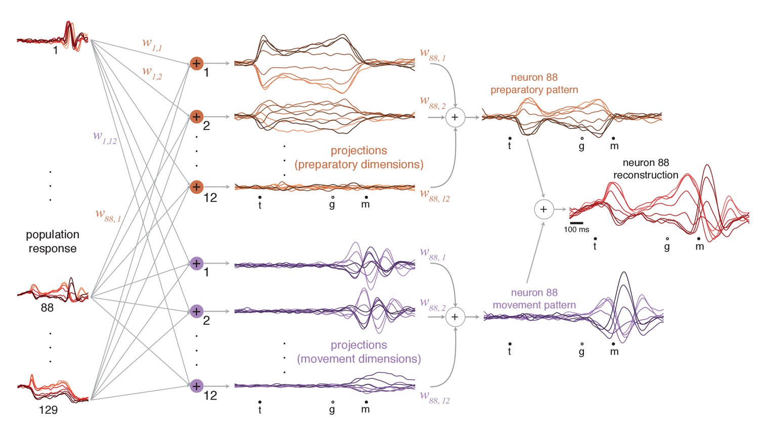
Illustration of how preparatory and movement-subspace projections were found using the cue-initiated context.
The population of neural responses (left column) can be linearly ‘read out’ into preparatory and movement-related projections (middle column). is the readout weight from the neuron to the projection, and the collection of such weights is the neural dimension. Because the identified dimensions maximize the variance captured, individual-neuron responses can be reconstructed from the projections. Reconstruction employs the same weights that defined the projections. For example, if neuron 88 contributed to the first preparatory projection with weight , then that first preparatory projection contributes to the reconstruction of neuron 88 with the same weight. The weighted sum of the preparatory projections yields that neuron’s ‘preparatory pattern’ (orange traces in right column). The weighted sum of movement projections yields that neuron’s ‘movement pattern’ (purple traces in right column). The full reconstruction is the sum of these two patterns, which describe the tuned aspects of the neuron’s response, plus a time-varying mean that captures any untuned trends in the overall mean firing rate with time (not shown). The success of the reconstruction can be appreciated by comparison with the true response in Figure 5a.
Figure 7
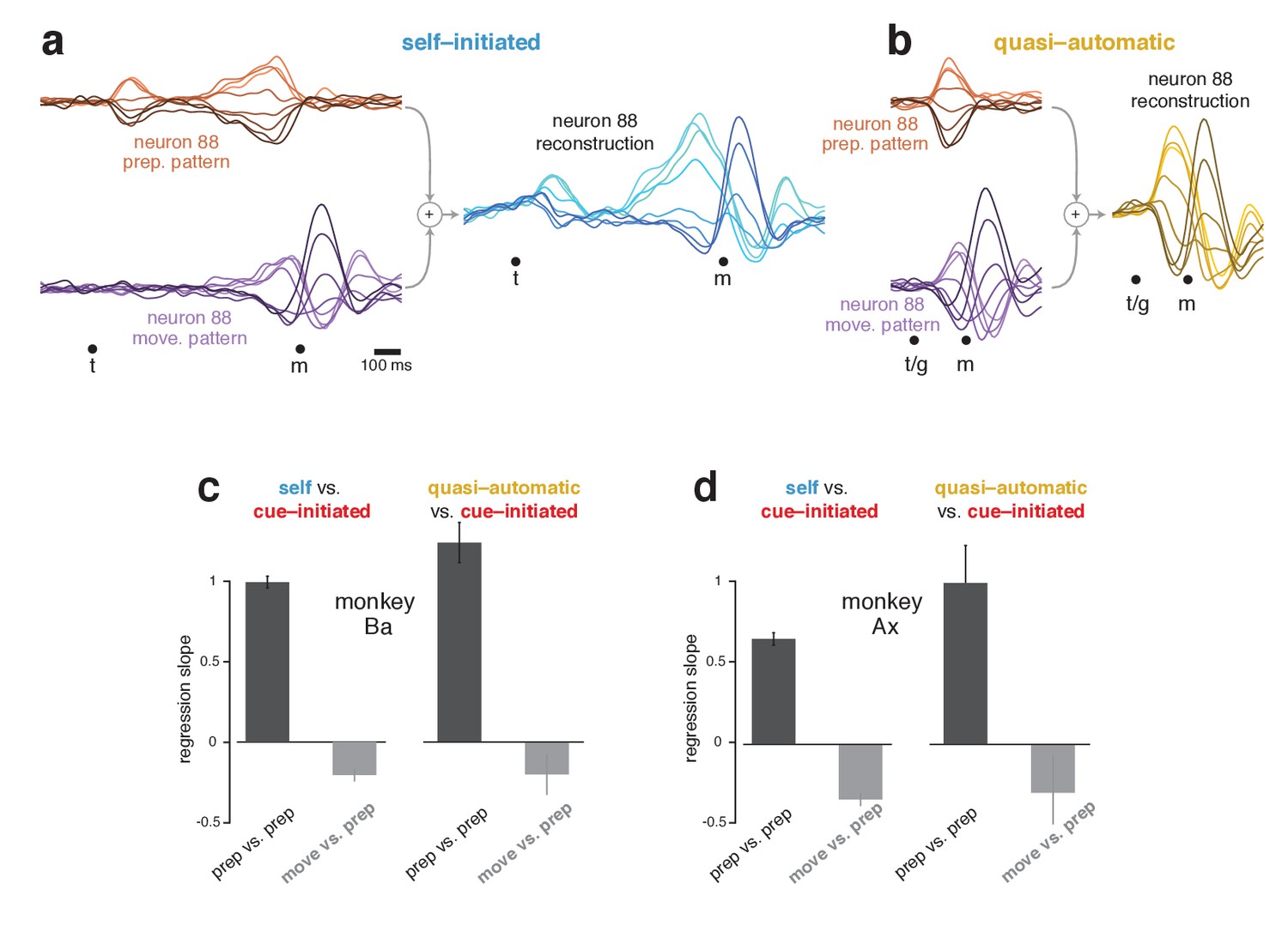
Reconstruction of single-neuron responses in the self-initiated and quasi-automatic contexts.
(a) Example reconstruction for the self-initiated context. The population response was projected onto the preparatory and movement dimensions, found using the cue-initiated context. We then used those projections to reconstruct the preparatory (orange) and movement (purple) patterns that contributed to each neuron’s response. These patterns are shown for neuron 88. The full reconstruction (blue) is the sum of the preparatory and movement patterns, plus the across-condition mean response (which has no tuning, but captures the overall mean rate at each time). This reconstructed response can be compared with the true response in Figure 5a. (b) As in (a), but for the quasi-automatic context. (c) Analysis of whether a neuron’s preparatory-subspace pattern exhibits similar ‘tuning’ across contexts. For each neuron, we took the value of the preparatory subspace pattern, 100 ms before movement onset, for each direction. These values form a vector with one element per direction. To compute the similarity of the vector for the self-initiated context with that for the cue-initiated context, we regressed the former versus the latter and took the slope. The same was done for the quasi-automatic context versus the cue-initiated context. Dark bars show the average slope across neurons ± SEM. As a comparison, we repeated this analysis but regressed the movement pattern during the self-initiated and quasi-automatic contexts versus the preparatory pattern during the cue-initiated context (light gray bars). The movement pattern was assessed 150 ms after movement onset. Data are for monkey Ba. (d) As in (c), but for monkey Ax.
Figure 8 with 1 supplement
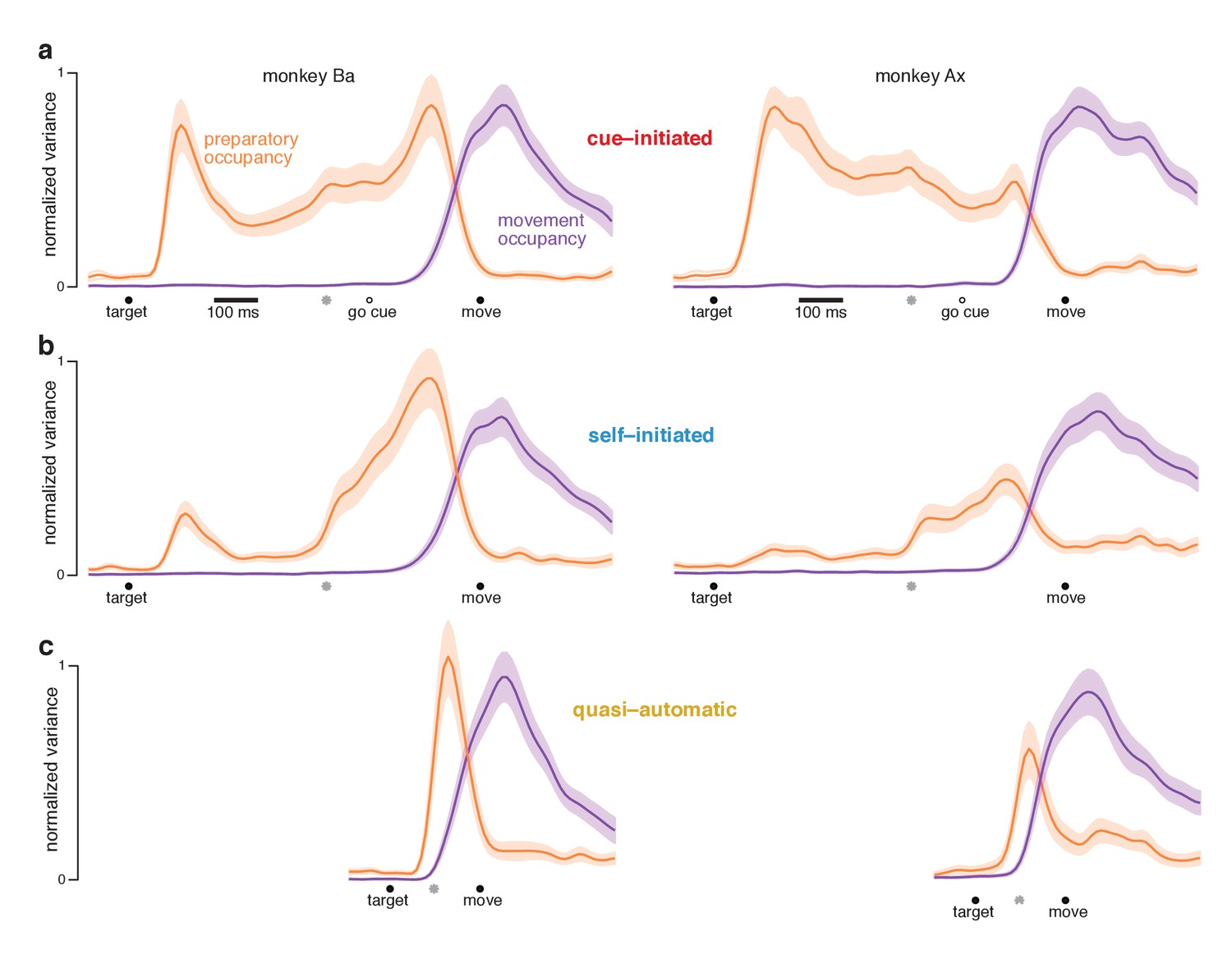
Preparatory and movement–subspace occupancy.
(a) Preparatory and movement subspace occupancy for the cue–initiated context. The two columns show results for monkeys Ba and Ax. Preparatory-subspace occupancy, across all three contexts, was normalized by the highest value attained in the cue-initiated context. Movement-subspace occupancy was similarly normalized. The shaded region denotes the standard deviation of the sampling error (equivalent to the standard error of the mean) computed via bootstrap. Gray symbols indicate the time when target-locked data and movement-locked data were concatenated. Open circle indicates the average time of the go cue relative to movement onset. (b,c) Occupancy during the self-initiated and quasi-automatic contexts respectively.
Figure 8—figure supplement 1
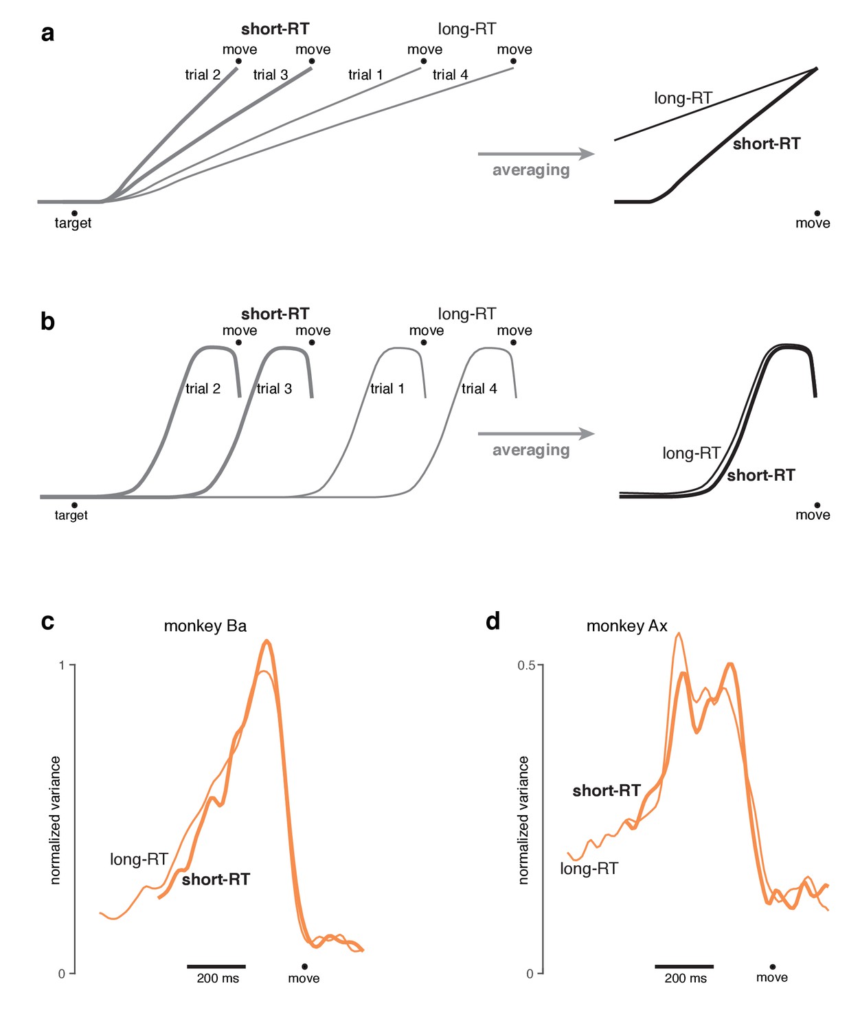
Testing predictions of different hypotheses regarding the development of preparatory activity on single trials in the self-initiated context.
(a) Schematic of the ‘target-locked-rise’ hypothesis. Under this hypothesis, preparatory activity develops shortly after target onset, but rises at different rates on different trials, leading to different RTs. A related hypothesis (not illustrated) is that the rise is stochastic and a higher average slope produces short RT trials. These hypotheses lead to the following prediction when trials are aligned to movement onset and averaged: when looking back in time, preparatory activity should decline slowly for trials with longer RTs (which had shallower slopes), and quickly for trials with shorter RTs (which had steeper slopes). (b) Schematic of the ‘prepare-on-demand’ hypothesis. Under this hypothesis, preparatory activity stays weak until close to the time of movement. Activity then rises in a stereotyped profile, and movement onset follows shortly thereafter. Note that this profile could involve a step, a ramp, or a variety of other shapes. The key aspect of this hypothesis is not the exact temporal profile, but rather the proposition that the profile is stereotyped across trials. Despite this stereotypy, average target-locked data could appear as a steady rise. In contrast, averages locked to movement onset would better capture the typical temporal profile. Thus, a central prediction of the prepare-on-demand hypothesis is that movement-locked averages will look similar for short-RT and long-RT trials. (c) Preparatory subspace occupancy computed from data locked to movement onset for monkey Ba. For each neuron, trials were divided into those shorter and longer than the median. This yielded both a short-RT and a long-RT population response. Populations responses were projected into the preparatory subspace (found using the cue-initiated context, as in Figure 8) and occupancy was computed. Only data after target onset are shown. Thus, the leftwards extent of each trace is limited by the longest interval between target onset and movement onset (which is of course longer for long-RT trials). The profile of preparatory occupancy is similar for short-RT and long-RT trials. These results are most consistent with the prepare-on-demand hypothesis. There is only a slight hint of occupancy being higher for long-RT trials prior to movement onset, as predicted by the target-locked-rise hypothesis. (d) Same as panel c but for monkey Ax. In summary, temporal profiles were somewhat different for the two monkeys (more ramp-like for monkey Ba and more step-like for monkey Ax). However, in both cases the profile was very similar regardless of RT, consistent with the prepare-on-demand hypothesis. We stress that this analysis still averages over potentially diverse single-trial events. For example, the ramp of preparatory subspace occupancy that begins ~400 ms before movement onset could be a ramp on every trial, or a step with somewhat variable timing: sometimes rising 350 ms before movement onset and sometimes rising 200 ms before movement onset. What can be concluded is that RT variability is not primarily driven by variability in the slope of ramping preparatory activity.
Figure 9
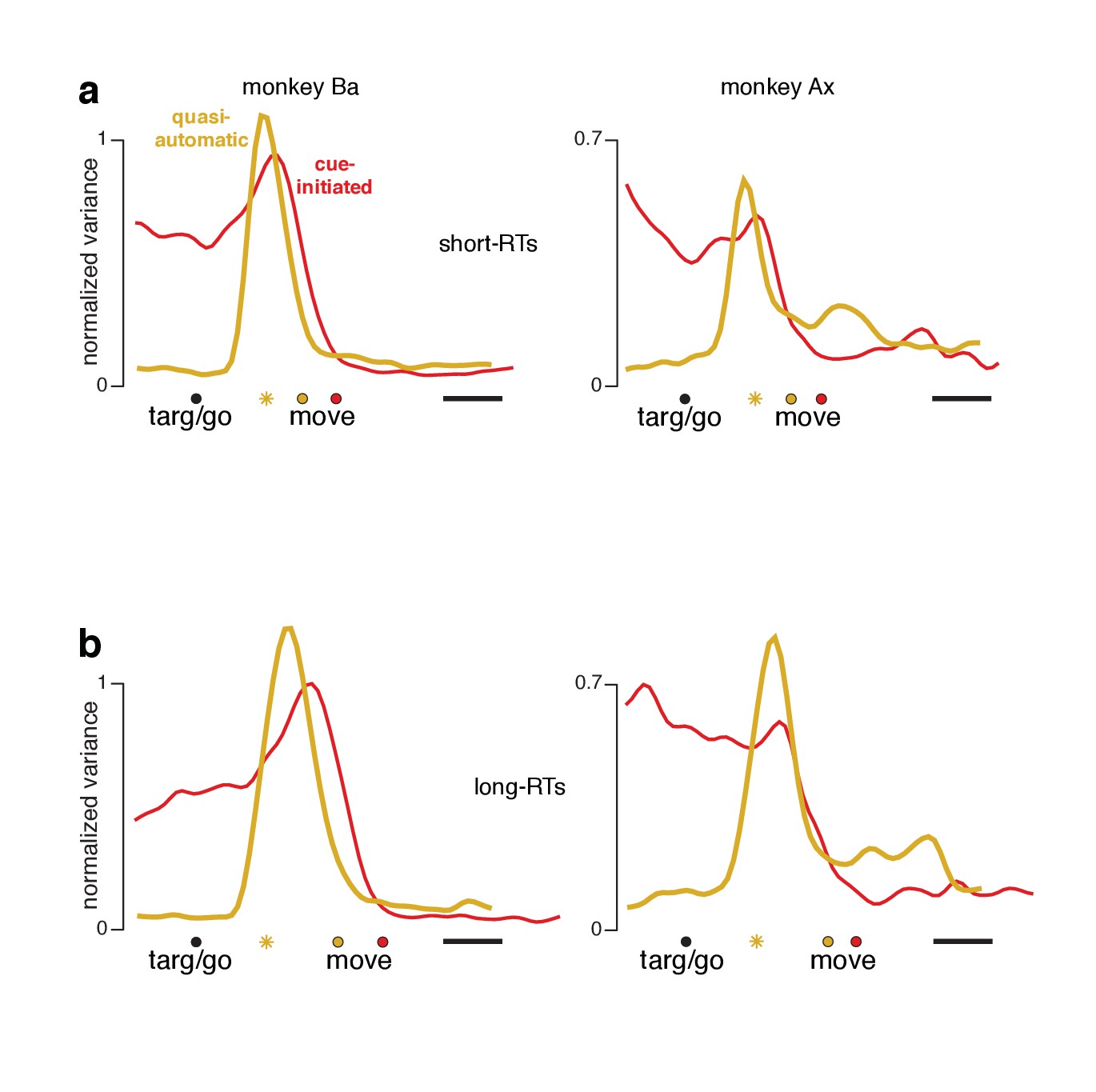
Preparatory-subspace occupancy for cue-initiated versus quasi-automatic contexts, after dividing trials by RT.
(a) Data for trials with RTs shorter than the median. We computed the mean firing rate of each neuron for trials with RTs shorter than the median for that context. The population was then projected onto the same preparatory-subspace dimensions employed in Figure 8. Data are aligned so that target onset for the quasi-automatic context is aligned with the go cue for the cue-initiated context (black circle). Colored circles indicate the time of movement onset for the analyzed trials. This occurs earlier for the quasi-automatic context (yellow circle) relative to the cue-initiated context (red circle) due to the shorter RTs in the quasi-automatic context. Horizontal scale bar indicates 100 ms. Yellow star indicates the moment of concatenation for the quasi-automatic context. (b) Same analysis but for trials with RTs longer than the median. These longer RTs are reflected in the rightward-shifted time of movement onset relative to target onset/the go cue. The concatenated timespans have been adjusted to reflect the different separation between target and movement onset for short- and long-RT trials.
Figure 10 with 2 supplements
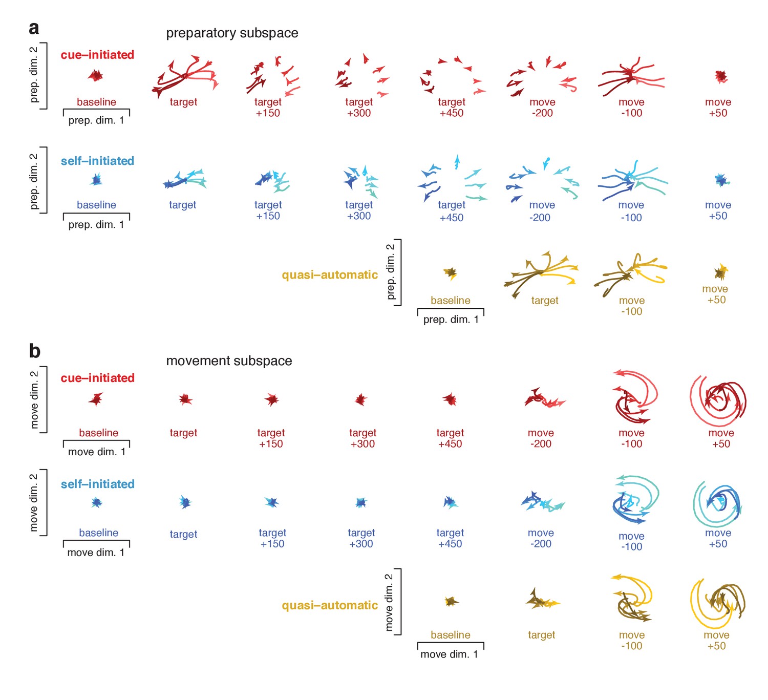
Snapshots of neural states in the preparatory and movement subspaces.
Responses for cue–initiated (red), self–initiated (blue) and quasi–automatic (yellow) contexts projected onto the top two preparatory dimensions (a) and top two movement dimensions (b) Trace-shading corresponds to target direction (same color scheme as in Figure 5). Each snapshot shows the neural state in that subspace, for all eight directions, during a 150 ms window. Snapshots labeled ‘baseline’ begin 150 ms before target onset. Snapshots labeled ‘target’ plot data starting at target onset. For the cue–initiated and self–initiated contexts, the subsequent three snapshots show activity in 150 ms increments, still aligned to target onset. Snapshots labeled ‘move −200’ start 200 ms before movement onset, with data aligned to movement onset. Subsequent panels begin at the indicated time. Data are for monkey Ba.
Figure 10—figure supplement 1
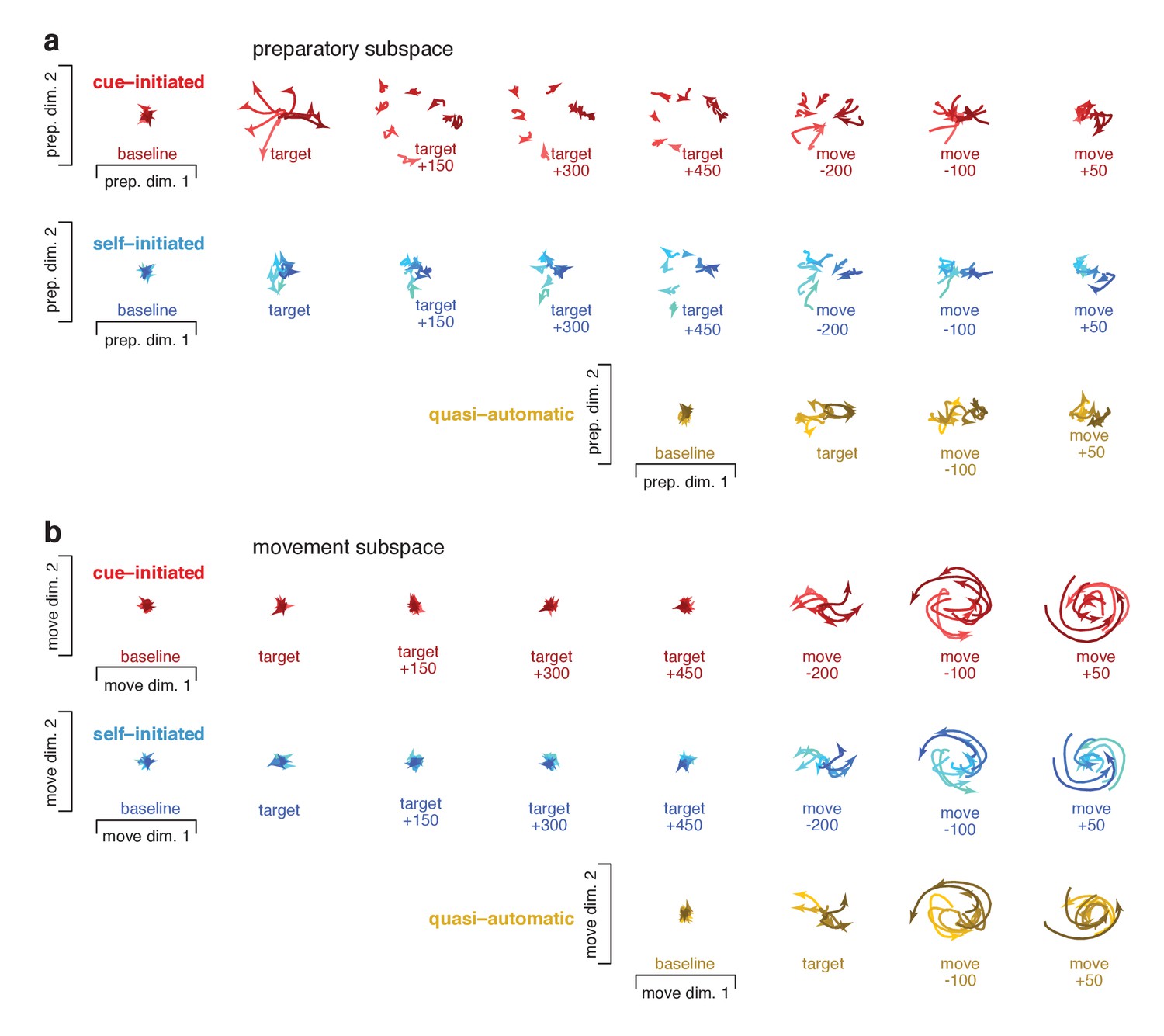
Snapshots of neural states in the preparatory and movement subspaces for monkey Ax.
All plotting conventions are as in Figure 10.
Figure 10—figure supplement 2
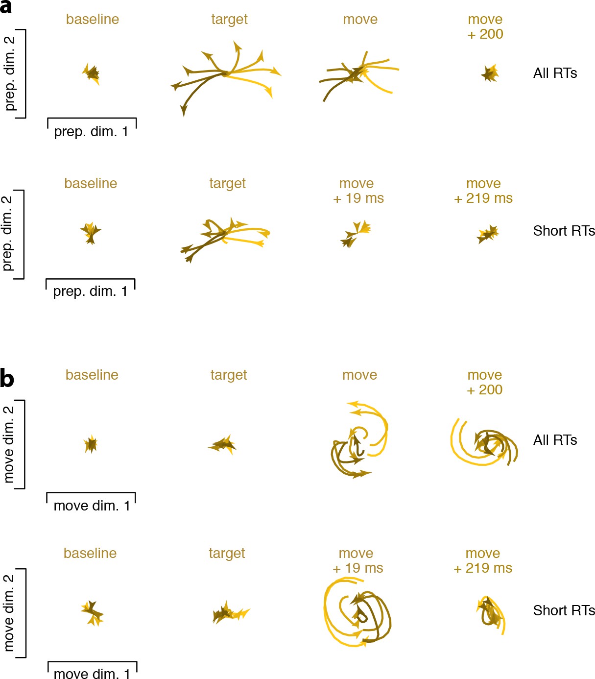
Snapshots of neural states comparing, for the quasi-automatic context, all trials with short-RT trials.
All projections are onto the same dimensions as in Figure 10. Each subpanel plots the evolution of activity over a 150 ms window. (a) Preparatory-subspace activity. Top row is reproduced from Figure 10. Bottom row is for trials with RTs shorter than the median. (b) Movement-subspace activity. Same conventions as for panel (a). Analysis windows have the same temporal alignment, relative to target onset, for all trials and for short-RT trials. Thus, the last two subpanels occur earlier, relative to movement onset, for short-RT trials (by the average RT difference of 19 ms). This allows one to observe that some key events occur more swiftly for short-RT trials. For the averages made from all trials, preparatory-subspace activity is just reaching its zenith at the end of the window starting at target onset. In contrast, for short-RT trials, activity has already begun to decline, in anticipation of movement onset, by the end of that window. This decline then completes sooner for short-RT trials (compare third subpanel across rows in a). Rotational dynamics also begin and end at earlier times for short-RT trials. This earlier occurrence of key events is expected, assuming a relatively tight link between the offset of preparatory-subspace activity, the onset of rotational dynamics, and the onset of muscle activity and physical movement. Note also that preparatory-subspace activity is truncated slightly earlier (and thus reaches a slightly lower peak magnitude) for short-RT trials. This accounts for the seemingly paradoxical finding that short-RT trials are associated with slightly lower, rather than higher, peak preparatory-subspace occupancy.
Figure 11 with 1 supplement
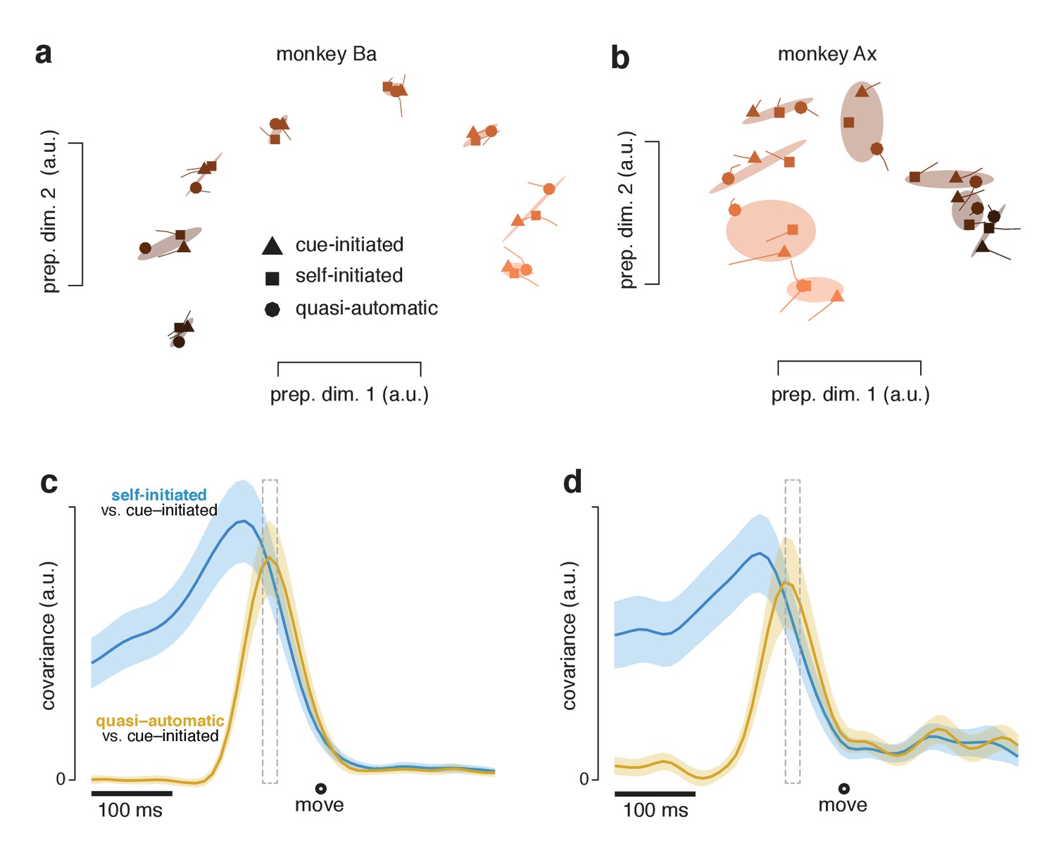
Preparatory subspace activity just before movement onset.
(a) Data for monkey Ba. Each marker denotes the neural state in the two preparatory dimensions that captured the most variance, as in Figure 10a. Markers indicate the state 55 ms before movement onset. Tails plot 20 ms of activity leading up to that time. The three shapes show states for the three contexts. Shaded regions plot the covariance ellipse for each triplet of states. A different symbol shade is used for each target direction (light for right, dark for left). (b) As in (a) but for monkey Ax. (c) Quantification of the time-course of the similarity in the pattern of preparatory states between contexts. Blue trace plots the covariance between the preparatory pattern in the self-initiated context and that in the cue-initiated context. Yellow trace plots the covariance between the preparatory pattern in the quasi-automatic context and that in the cue-initiated context. The covariance is high when patterns are both strong and similar. The vertical scale is arbitrary (for reference, the correlation peaks close to one). Correlations are computed using all 12 preparatory dimensions. Results are very similar when considering only the top two dimensions. Gray dashed window of time indicates the 20 ms time range (from 75 to 55 ms before movement onset) shown in (a). The shaded regions denote the standard deviation of the sampling error (equivalent to the standard error) computed via bootstrap. Data are from monkey Ba. (d) As in panel c, but for monkey Ax.
Figure 11—figure supplement 1
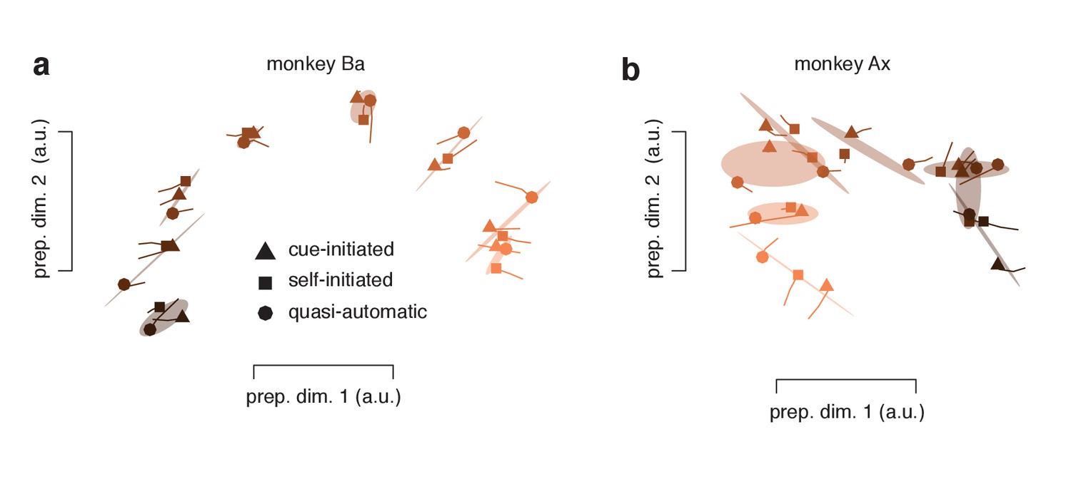
Same analysis as in Figure 11a,b but after restricting analysis to trials with RTs shorter than the median.
Restriction was performed (separately) for all three contexts. Data are projected onto the same dimensions used in Figure 11. Two observations can be made. First, it is not the case that preparatory-subspace structure becomes absent for short-RT quasi-automatic trials. For such trials, the preparatory-subspace state still varies strongly across target locations (different colored circles). This observation further underscores the results obtained when analyzing occupancy (Figure 9a). Second, preparatory-subspace states continue to cluster by target direction. That is, for a given target direction, the preparatory states for the three contexts tend to be close to one another. Clustering is slightly weaker than when considering all the data (Figure 11a,b). This may be a real effect or may simply reflect increased sampling noise after down-selection (some neurons are now contributing only 3 trials for a given target location).
Author response image 1
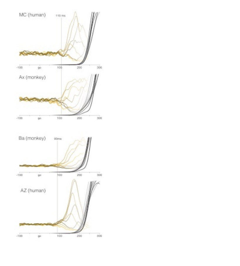
Comparison of EMG between humans and monkeys.
All data are for the quasi-automatic context. MC and AZ are two of the authors. Yellow traces show average target-locked EMG for all eight target directions. Latency is estimated manually as the first moment when activity begins to separate for the different directions. Recordings are from the deltoid. We chose the deltoid as the most natural point of comparison because the shoulder was the primary joint responsible for producing the reach. The deltoid had a ‘smooth’ onset: initially changing slowly and then more rapidly. Other muscles (e.g., the biceps) had a more abrupt onset. Average target-locked hand velocity is shown by gray-to-black shaded traces (one per target direction). One might have expected EMG onset to be later in humans given the greater length of cortico-spinal axons. However, conduction velocities in the corticospinal tract are very fast (exceeding 100 m/s).
Tables
Table 1
Rates of different categories of task error.
Percentages consider trials that were successfully initiated (i.e. the monkey held the touch point and a target appeared) but were subsequently failed. The target was missed if a reach was executed but did not land within the acceptance window. Delay violations occurred if above-threshold hand velocity was detected between target onset and the go cue. This could occur if the monkey made an overt reach or a small adjustment. Trials were also failed if hand velocity was above threshold during the interval from the go cue until 100 ms later. Changes in hand velocity during this time are unlikely to reflect legitimate responses to the go cue, and were thus treated the same way as movement during the delay. Movement during the target-hold period (after it was successfully hit) also resulted in a failure. This occurred if velocity exceeded threshold, or if hand position exited the acceptance window. The maximum RT (500 ms for cue-initiated, 1500 ms for self-initiated) elapsed if the hand never moved. Such failures tended to happen if the monkey became distracted during a trial, or near the end of the day as motivation waned. For example, simply holding the hand on the screen but not performing the task resulted in such failures being recorded. Violations of the maximum movement duration occurred if the hand left the touch-point but did not land on the target within 500 ms. This could occur for very sluggish movements, or if the monkey simply aborted the trial and did not attempt to hit the target. We also included in this category failures in the quasi-automatic context where the hand did not land back on the screen before the target disappeared off the screen.
| Monkey ba | Monkey ax | |||||
|---|---|---|---|---|---|---|
| Cue-initiated | Self-initiated | Quasi-automatic | Cue-initiated | Self-initiated | Quasi-automatic | |
| Missed target | 1.4% | 4.1% | 3.3% | 0.9% | 1.6% | 2.4% |
| Delay violation (adjustment or overt reach) | 2.2% | NA | NA | 1.3% | NA | NA |
| Velocity violation within 100 ms of go cue (adjustment or non-physiological RT) | 1.6% | 0.1% | 0.6% | 1.1% | 0% | 0.5% |
| Moved during target-hold period | 1.4% | 1.3% | 2.1% | 1.5% | 1.2% | 1.1% |
| Max RT elapsed | 2.2% | 2.6% | NA | 0.8% | 0.6% | NA |
| Max movement duration elapsed | 0.2% | 0.2% | 1.3% (target left screen) | 0.1% | 0.2% | 2.7% (target left screen) |
Table 2
Significance tests for features of the time-course of preparatory subspace occupancy.
P-values were computed via bootstrap. Neurons were redrawn and the central analysis (computing subspaces etc.) was performed again for the redrawn population. This process was repeated 1000 times, and the relevant measure was made, yielding a sampling distribution of 1000 values. P-values were based on these sampling distributions.
| Monkey ba | Monkey ax | |
|---|---|---|
| Prep. occ. declines before movement onset. (150 ms before vs. 150 ms after move onset, cue-initiated) | p<0.001 | p<0.001 |
| Target-driven rise in prep. occ. is smaller for self- vs. cue-initiated (compared 150 ms after target onset) | p<0.001 | p<0.001 |
| Self-initiated prep. occ. remains above baseline after post-target peak (400 ms post-target vs 150 ms pre-target) | p<0.001 | p<0.001 |
| Self-initiated prep. occ. grows as movement approaches (150 ms before move onset vs 150 ms after target onset) | p<0.001 | p<0.001 |
| Prep. occ. before movement onset is similar but slightly different for self- and cue-initiated contexts (assessed 150 ms before move onset) | p<0.003 (larger for self-) | N.S. (smaller for self-) |
| Prep. occ. rises above baseline in the quasi-automatic context | p<0.001 | p<0.001 |
| Pre-movement peak in prep. occ. is modestly higher for quasi-automatic context versus other two contexts | p<0.002 for both comparisons | p<0.002 for both comparisons |
| Prep. occ. precedes move. occ . even for quasi-automatic context (compare latency to cross threshold set to 10% of peak) | p<0.001 | p<0.001 |
Additional files
-
Transparent reporting form
- https://doi.org/10.7554/eLife.31826.024
Download links
A two-part list of links to download the article, or parts of the article, in various formats.
Downloads (link to download the article as PDF)
Open citations (links to open the citations from this article in various online reference manager services)
Cite this article (links to download the citations from this article in formats compatible with various reference manager tools)
Conservation of preparatory neural events in monkey motor cortex regardless of how movement is initiated
eLife 7:e31826.
https://doi.org/10.7554/eLife.31826


