Figures and data in Adaptive coding for dynamic sensory inference | eLife

Figures
Additional files

7 figures and 1 additional file

Figures

Figure 1 with 2 supplements

Download asset Open asset

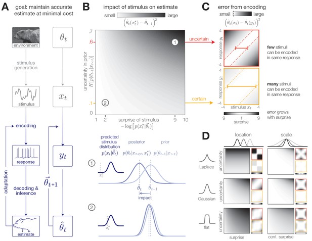
Surprise and uncertainty determine the impact of incoming stimuli for efficient inference.

(A) We consider a framework in which a sensory system infers the state of a dynamic environment at minimal metabolic cost. The state of the environment ( $θ_{t}$ ) is signaled by sensory stimuli ( $x_{t}$ ) that are encoded in neural responses ( $y_{t}$ ). To infer this state, the system must decode stimuli from neural responses and use them to update an internal model of the environment (consisting of an estimate ${\hat{θ}}_{t}$ and a prediction ${\vec{θ}}_{t + 1}$ ). This internal model can then be used to adapt the encoding at earlier stages. (The image of the bear was taken from the Berkeley Segmentation Dataset, Martin et al., 2001). (B) Incoming stimuli can have varying impact on the observer’s estimate of the environmental state depending on the relationship between the observer’s uncertainty and the surprise of the stimulus (heatmap). We use the example of Bayesian estimation of the mean of a stationary Gaussian distribution (Murphy, 2007) to demonstrate that when the observer is uncertain (wide prior $p (θ_{t - 1} | x_{τ < t})$ ) and the stimulus $x_{t}^{*}$ is surprising ( $x_{t}^{*}$ falls on the edge of the distribution $p (x_{t} | {\vec{θ}}_{t})$ ), the stimulus has high impact and causes a large shift in the posterior $p (θ_{t} | x_{t}^{*}, x_{τ < t})$ (schematic (1)). In contrast, when the observer is certain and the stimulus is expected, the stimulus has a small impact on the observer’s estimate (schematic (2)). We quantify impact by the squared difference ${(\hat{θ} (x_{t}^{*}) - {\hat{θ}}_{t - 1})}^{2}$ between the estimate before and after incorporating the stimulus (Materials and methods). (Computed using ${\hat{θ}}_{t - 1} = 0$ , for which impact spans the interval [0,0.7]). (C) When the observer is certain, a large number of stimuli can be mapped onto the same neural response without inducing error into the observer’s estimate (orange panel). When the observer is uncertain, the same mapping from stimulus to response induces higher error (red panel). Error is highest when mapping a surprising stimulus onto an expected neural response, or vice versa. We quantify error by the squared difference ${({\hat{θ}}_{t} (x_{t}) - {\hat{θ}}_{t} (y_{t}))}^{2}$ between the estimate constructed with the stimulus versus the response (Materials and methods). Shown for uncertainty values of 0.1 (orange) and 0.6 (red). Pairs of colored dotted lines superimposed on the heatmap indicate contours of constant error tolerance $E_{t o l} = 0.05$ (whose value is also marked by the vertical dotted line in the colorbar). Colored horizontal bars indicate the set of stimuli ${x_{t}}$ that can be mapped to the same neural response $y_{t} = 0$ with an error less than $E_{t o l}$ . (D) Qualitatively similar results to those shown in panels B-C are observed for estimating the location and scale of a stationary generalized Gaussian distribution. Stimuli have a larger impact on the observer’s estimate when the observer is uncertain and when stimuli are unexpected (quantified by surprise in the case of location estimation, and centered surprise in the case of scale estimation; see main text). The error induced by mapping a stimulus onto a response grows with the surprise of the stimulus. For the case of scale estimation, this error is symmetric to exchanging $+ x$ and $- x$ , because positive and negative deviations from the mean (taken here to be 0) exert similar influence on the estimation of scale. Results are computed using ${\hat{θ}}_{t - 1} = 0$ (location) and ${\hat{θ}}_{t - 1} = 1$ (scale) and are displayed over the same ranges of uncertainty ([0,0.7]), surprise/centered surprise (Yu et al., 2015; Roddey et al., 2000), and stimulus/response ([−4,4]) as in panels B-C. Heatmaps of impact are individually scaled for each stimulus distribution relative to their minimum and maximum values; heatmaps of encoding error are scaled relative to the minimum and maximum error across both uncertainty values for a given stimulus distribution. See Figure 1—figure supplement 2 for numerical values of color scale.

https://doi.org/10.7554/eLife.32055.002

Figure 1—figure supplement 1

Download asset Open asset

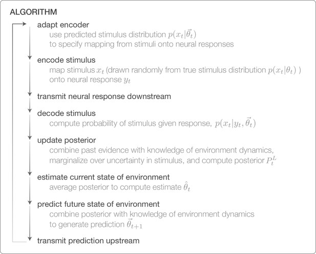
Algorithm for performing Bayesian inference with adaptively encoded stimuli.
https://doi.org/10.7554/eLife.32055.003

Figure 1—figure supplement 2

Download asset Open asset

Minimum and maximum values of the color ranges shown in Figure 1B–D.
https://doi.org/10.7554/eLife.32055.004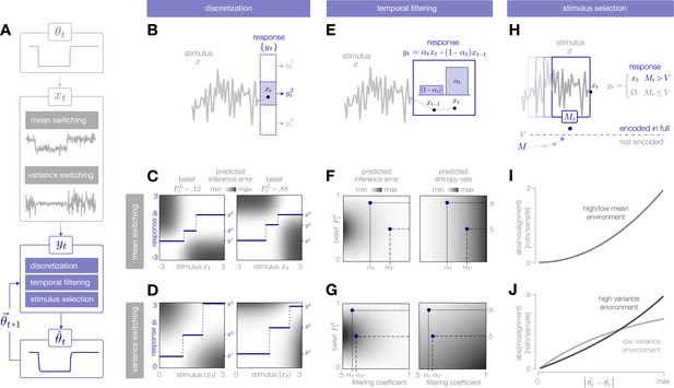

Figure 2 with 1 supplement

Download asset Open asset

Adaptive encoding schemes.

(A) We consider a specific implementation of our general framework in which an environmental state $θ_{t}$ switches between two values with fixed probability. This state parameterizes the mean or variance of a Gaussian stimulus distribution. Stimuli $x_{t}$ are drawn from this distribution and encoded in neural responses $y_{t}$ . We consider three encoding schemes that perform discretization (panels B-D), temporal filtering (panels E-G), or stimulus selection (panels H-J) on incoming stimuli. (B) (Schematic) At each timestep, an incoming stimulus $x_{t}$ (black dot) is mapped onto a discrete neural response level $y_{t}^{i}$ (solid blue rectangle) chosen from a set ${y_{t}^{i}}$ (dotted rectangles). (C–D) The predicted inference error induced by mapping a stimulus $x_{t}$ onto a neural response $y_{t}$ varies as a function of the observer’s belief $P_{t}^{L}$ about the state of the environment (shown for $P_{t}^{L} = 0.12$ , left column; $P_{t}^{L} = 0.88$ , right column). At each timestep, the optimal response levels ${y^{1}, y^{2}, y^{3}}$ (solid lines) are chosen to minimize this error when averaged over the predicted stimulus distribution. See Figure 2—figure supplement 1A for numerical values of color scale. (E) (Schematic) At each timestep, incoming stimuli are combined via a linear filter with a coefficient $α_{t}$ . (F–G) The average predicted inference error (left column) depends on the filter coefficient $α_{t}$ and on the observer’s belief $P_{t}^{L}$ about the state of the environment. At each timestep, the optimal filter coefficient (blue dot) is found by balancing error and entropy given a prediction of the environmental state ( $α_{t}$ and $α_{t^{'}}$ are shown for $P_{t}^{L} = 0.9$ and $P_{t^{'}}^{L} = 0.5$ , respectively). See Figure 2—figure supplement 1B for numerical values of color scale. (H) (Schematic) At each timestep, the encoder computes the misalignment $M_{t}$ between the predicted and measured surprise of incoming stimuli. If the misalignment exceeds a threshold $V$ , the stimulus is encoded with perfect fidelity; otherwise, the stimulus is not encoded. (I–J) The misalignment signal (computed here analytically; see Materials and methods) depends on the relationship between the predicted and true state of the environment. When the mean is changing over time (panel I), the misalignment depends only on the absolute difference between the true and predicted mean. When the variance is changing over time (panel J), the misalignment also depends on the true variance of the environment.

https://doi.org/10.7554/eLife.32055.005

Figure 2—figure supplement 1

Download asset Open asset

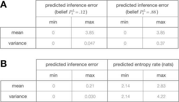
Minimum and maximum values of the color ranges shown in Figure 2.

Each entry reports the minimum or maximum value of (A) the predicted inference error induced by discretization (as shown in Figure 2C–D), or (B) the predicted inference error or predicted entropy rate induced by filtering (as shown in Figure 2F–G).

https://doi.org/10.7554/eLife.32055.006

Figure 3 with 2 supplements

Download asset Open asset

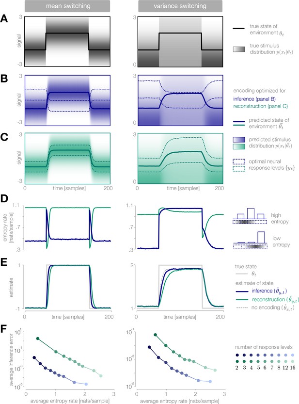
Dynamic inference with optimally-adapted response levels.

(A) We consider a probe environment in which a state $θ_{t}$ (solid line) switches between two values at fixed time intervals. This state parametrizes the mean (left) or the variance (right) of a Gaussian stimulus distribution (heatmap). (B, C) Optimal response levels (dotted lines) are chosen to minimize error in inference (blue) or stimulus reconstruction (green) based on the predicted stimulus distribution $p (x_{t} | {\vec{θ}}_{t})$ (heatmap). Results are shown for three response levels. All probability distributions in panels A-C are scaled to the same range, $[0, 0.4]$ . (B) Response levels optimized for inference devote higher resolution (narrower levels) to stimuli that are surprising given the current prediction of the environment. (C) Response levels optimized for stimulus reconstruction devote higher resolution to stimuli that are likely. (D) The entropy rate of the encoding is found by partitioning the true stimulus distribution (heatmap in panel A) based on the optimal response levels (dotted lines in panels B-C). Abrupt changes in the environment induce large changes in entropy rate that are symmetric for mean estimation (left) but asymmetric for variance estimation (right). Apparent differences in the baseline entropy rate for low- versus high-mean states arise from numerical instabilities. (E) Encoding induces error in the estimate ${\hat{θ}}_{t}$ . Errors are larger if the encoding is optimized for stimulus reconstruction than for inference. The error induced by upward and downward switches is symmetric for mean estimation (left) but asymmetric for variance estimation (right). In the latter case, errors are larger when inferring upward switches in variance. (F) Increasing the number of response levels decreases the average inference error but increases the cost of encoding. Across all numbers of response levels, an encoding optimized for inference (blue) achieves lower error at lower cost than an encoding optimized for stimulus reconstruction (green). All results in panels A-C and E are averaged over 500 cycles of the probe environment. Results in panel D were computed using the average response levels shown in panels B-C. Results in panel F were determined by computing time-averages of the results in panels D-E.

https://doi.org/10.7554/eLife.32055.007

Figure 3—figure supplement 1

Download asset Open asset

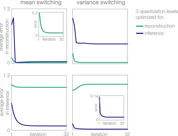
Learning of optimal response levels with Lloyd’s algorithm.

Optimization of three response levels (quantization levels) for reconstruction (green) differs from optimization for inference (blue). Regardless of the error function (distortion measure), the algorithm converges to an optimum.

https://doi.org/10.7554/eLife.32055.008

Figure 3—figure supplement 2

Download asset Open asset

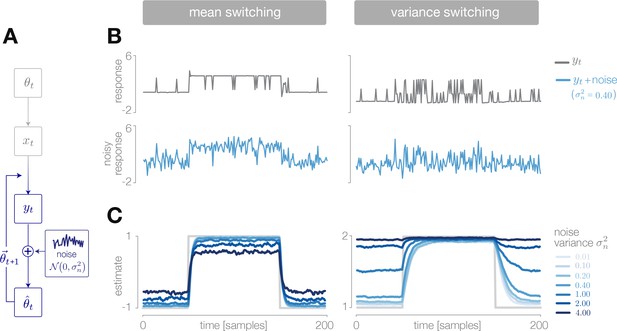
Deviations from optimal inference due to transmission noise.

(A) We simulated the noisy transmission of stimulus representations to downstream areas by injecting additive Gaussian noise into the response of a discretizing encoder. (B) The output response $y_{t}$ of the encoder is a discretized version of the incoming stimulus (upper row, gray). The observer receives a noisy version of the response (lower row, blue). (C) The estimate ${\hat{θ}}_{t}$ is robust at low-noise levels, but degrades significantly for high noise levels. Results are averaged over 500 cycles of the probe environment.

https://doi.org/10.7554/eLife.32055.009

Figure 4

Download asset Open asset

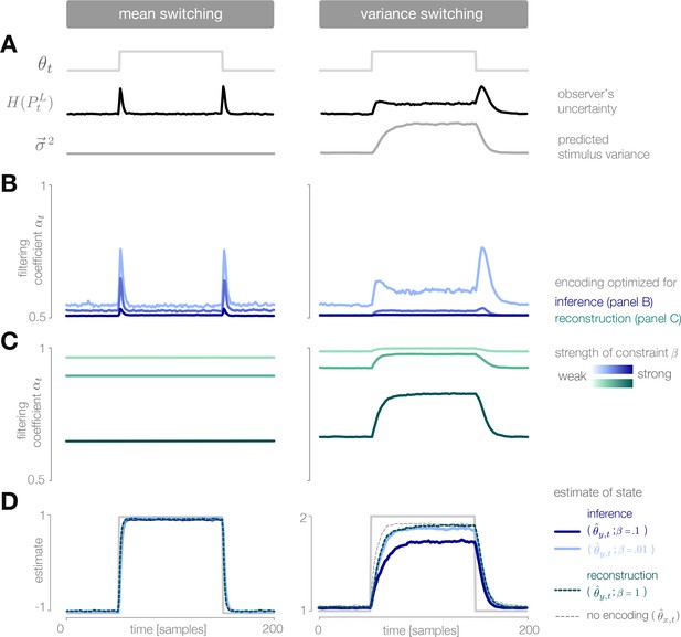
Dynamic inference with optimally-adapted temporal filters.

(A) The observer’s uncertainty ( $H [P_{t}^{L}]$ ) is largest when the environment is changing. The predicted stimulus variance (a proxy for both the predicted magnitude of the stimulus distribution, and the predicted surprise of incoming stimuli) is constant in a mean-switching environment (left) but variable in a variance-switching environment (right) (computed using a filter coefficient optimized for inference with a weak entropy constraint, corresponding to the lightest blue curves in panel B). (B, C) Optimal values of the filter coefficient $α_{t}$ are chosen at each timestep to minimize error in inference (blue) or stimulus reconstruction (green), subject to a constraint on predicted entropy. Darker colors indicate stronger constraints. (B) Filters optimized for inference devote high fidelity at times when the observer is uncertain and stimuli are predicted to be surprising. Shown for $β = 0.02, 0.1, 1$ (left) and $β = 0.01, 0.1, 1$ (right). (C) Filters optimized for reconstruction devote fidelity at times when the magnitude of the stimulus is predicted to be high. Shown for $β = 0.01, 0.1, 1$ . (D) Filtering induces error into the estimate ${\hat{θ}}_{t}$ . Strong filtering has minimal impact on mean estimation (left), but induces large errors in the estimation of high variances (right). All results in panels A-D are averaged over 800 cycles of the probe environment.

https://doi.org/10.7554/eLife.32055.010

Figure 5

Download asset Open asset

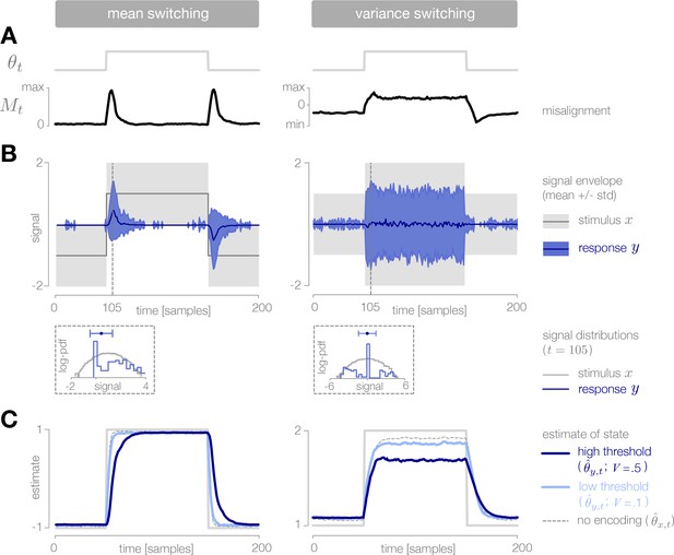
Dynamic inference with stimulus selection.

(A) When the environment is changing, the observer’s prediction is misaligned with the state of the environment. When this misalignment $M_{t}$ is large, stimuli are transmitted in full ( $y_{t} = x_{t}$ ). When this misalignment falls below a threshold $V$ , stimuli are not transmitted at all ( $y_{t} = 0$ ). (B) The distribution of encoded stimuli changes over time, as can be seen by comparing the envelope of the stimulus distribution (gray) with the envelope of the neural responses (blue). Left: When the mean of the stimulus distribution changes abruptly, a large proportion of stimuli are encoded, and the mean of the neural response (blue line) approaches the mean of the stimulus distribution (black line). At times when the mean of the stimulus distribution is stable, very few stimuli are encoded, and the mean of the neural response drops to zero. Right: When the variance is low, very few stimuli are encoded. When the variance increases, the average surprise of incoming stimuli increases, and a large proportion of stimuli are encoded. The envelope of the neural response expands and approaches the envelope of the stimulus distribution. Insets: At times when the environment is changing (shown for $t = 105$ ), the distribution of responses (blue) is sparser than the distribution of stimuli (gray), due to the large proportion of stimuli that are not encoded (indicated by the large peak in probability mass at $0$ ). Shown for $V = 0.5$ . (C) Higher thresholds slow the observer’s detection of changes in the mean (left), and cause the observer to underestimate high variances (right). Threshold values are scaled relative to the maximum analytical value of the misalignment signal in the mean- and variance-switching environment (shown in Figure 2I and J, respectively). Results in panels B and C are averaged over 800 cycles of the probe environment.

https://doi.org/10.7554/eLife.32055.011

Figure 6 with 1 supplement

Download asset Open asset

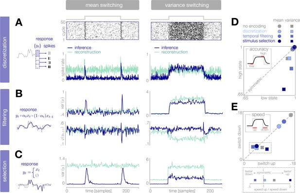
Dynamical signatures of adaptive coding schemes.

(A–C) We simulate the output of each encoder to repeated cycles of the probe environment. In the case of discretization (panel A), we use a simple entropy coding procedure to map optimal response levels ${y_{t}}$ onto spike patterns, as shown by the spike rasters. In the case of temporal filtering (panel B) and stimulus selection (panel C), we measure properties of the response $y_{t}$ . When encodings are optimized for inference (dark blue traces), abrupt changes in the mean of the stimulus distribution (panels A-C, left) are followed by transient increases in spike rate (discretization, panel A) and response variability (filtering, panel B; stimulus selection, panel C). In the case of temporal filtering, these changes are additionally marked by decreases in the temporal correlation $φ (y_{t, t + 1})$ of the response. In contrast, the response properties of encoders optimized for stimulus reconstruction (light green traces) remain more constant over time. Abrupt changes in variance (panels A-C, right) are marked by changes in baseline response properties. Responses show transient deviations away from baseline when encodings are optimized for inference, but remain fixed at baseline when encodings are optimized for reconstruction. In all cases, encodings optimized for inference maintain lower baseline firing rates, lower baseline variability, and higher baseline correlation than encodings optimized for stimulus reconstruction. Spike rates (panel A) are averaged over 500 cycles of the probe environment. Response variability (panels B-C) is computed at each timepoint across 800 cycles of the probe environment. Temporal correlation $φ (y_{t, t + 1})$ (panel B) is computed between consecutive timepoints across 800 cycles of the probe environment. (D–E) Encoding schemes impact both the accuracy (panel D) and speed (panel E) of inference. In all cases, the dynamics of inference are symmetric for changes in mean (points lie along the diagonal) but asymmetric for changes in variance (points lie off the diagonal). Encodings decrease the accuracy of estimating high-variance states (panel D), and they alter the speed of responding to changes in both mean and variance. The response to upward versus downward switches (dotted box) separates encoding schemes based on whether they are faster (right of dotted vertical line) or slower (left of dotted vertical line) to respond to increases versus decreases in variance. Speed and accuracy are measured from the trial-averaged trajectories of ${\hat{θ}}_{y, t}$ shown in Figure 3E, Figure 4D ( $β = 0.01$ ), and Figure 5C ( $V = 0.5$ ) (Materials and methods).

https://doi.org/10.7554/eLife.32055.012

Figure 6—figure supplement 1

Download asset Open asset

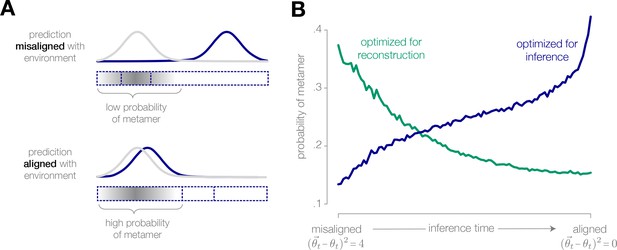
Physically different stimuli become indistinguishable to an adapted system optimized for inference.

(A) (Schematic) If the observer’s prediction is misaligned with the true state of the environment, the stimuli that are most likely to occur in the environment are mapped onto different neural responses. The probability of a metamer—defined by the set of stimuli that give rise to the same neural response—is low. Conversely, when the prediction is closely aligned with the environment, the probability of a metamer is high. (B) When an encoding is optimized for inference, the probability of a metamer increases as the observer’s prediction aligns with the environment, because an increasing fraction of stimuli are mapped onto the same neural response. The opposite trend is observed when the encoding is optimized for stimulus reconstruction (illustrated for a discretized encoder with eight response levels operating in a mean-switching environment).

https://doi.org/10.7554/eLife.32055.013

Figure 7 with 1 supplement

Download asset Open asset

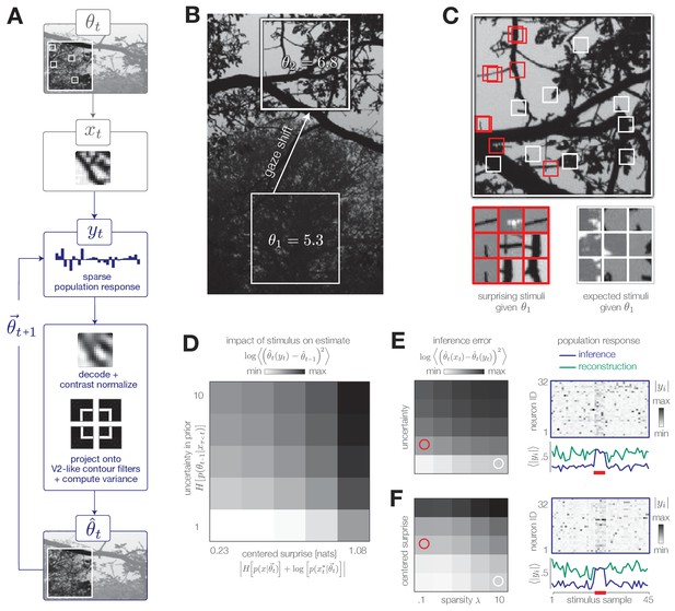
Model inference task with natural stimuli.

(A) We model a simple task of inferring the variance of local curvature in a region of an image. The system encodes randomly drawn image patches that model saccadic fixations. Individual image patches are encoded in sparse population activity via V1-like receptive fields (see Figure 7—figure supplement 1). Image patches are then decoded from the population activity, contrast-normalized, and projected onto V2-like curvature filters. The observer computes the variance of these filter outputs. (B) After a gaze shift from an area of low curvature (bottom square, $θ = θ_{1}$ ) to an area of high curvature (top square, $θ = θ_{2}$ ), the observer must update its estimate of local curvature. (C) Image patches that are surprising given the observer’s estimate (red) have larger variance in curvature, while expected patches (white) have low variance in curvature. Frames of highly overlapping patches were slightly shifted for display purposes. (D) Individual image patches have a large impact on the observer’s estimate when the observer is uncertain and when image patches have high centered surprise, analogous to the behavior observed in simple model environments (see Figure 1B). Shown for $λ = 0.1$ . Impact spans the interval [0, 34.12]. (E) The observer can exploit its uncertainty to adapt the sparsity of the sensory encoding (heatmap; blue trace). When the observer is certain (white marker), population activity can be significantly reduced without changing the inference error. Increases in uncertainty (red marker) result in bursts of activity (red bar). An encoder optimized for constant reconstruction error produces activity that remains constant over time (green trace). Inference error spans the interval [0, 2.22]. (F) The observer can similarly exploit the predicted surprise of incoming stimuli to reduce population activity when stimuli are expected. Inference error spans the interval [0, 1.57].

https://doi.org/10.7554/eLife.32055.014

Figure 7—figure supplement 1

Download asset Open asset

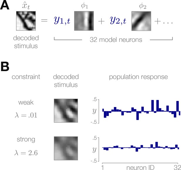
Sparse coding model of natural image patches.

(A) Each reconstructed image patch ${\hat{x}}_{t}$ is represented as a linear combination of basis functions $ϕ_{i}$ multiplied by sparse coefficients ${y_{i, t}}$ . (B) Small values of the sparsity constraint $λ$ (upper row) result in a more accurate reconstruction of the stimulus, but require a stronger population response to encode. Large values of $λ$ (bottom row) result in a weaker population response at the cost of decreased quality of the stimulus reconstruction.

https://doi.org/10.7554/eLife.32055.015

Additional files

Transparent reporting form: https://doi.org/10.7554/eLife.32055.016
Download elife-32055-transrepform-v1.pdf

Download links

A two-part list of links to download the article, or parts of the article, in various formats.

Downloads (link to download the article as PDF)

Open citations (links to open the citations from this article in various online reference manager services)

Mendeley

Cite this article (links to download the citations from this article in formats compatible with various reference manager tools)

Wiktor F Młynarski
Ann M Hermundstad

(2018)

Adaptive coding for dynamic sensory inference

eLife 7:e32055.

https://doi.org/10.7554/eLife.32055

Sign up for email alerts

Privacy notice