Single-exposure visual memory judgments are reflected in inferotemporal cortex
- University of Pennsylvania, United States
Figures
Figure 1
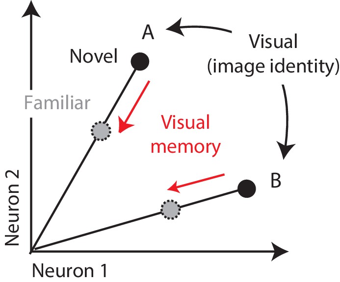
Multiplexing visual and visual memory representations.
Shown are the hypothetical population responses to two images (A and B), each presented as both novel and familiar, plotted as the spike count response of neuron 1 versus neuron 2. In this scenario, visual information (e.g. image or object identity) is reflected by the population response pattern, or equivalently, the angle that each population response vector points. In contrast, visual memory information is reflected by changes in population vector length (e.g. a multiplicative rescaling with stimulus repetition). Because visual memory does not impact vector angle in this hypothetical scenario, superimposing visual memories in this way would mitigate the impact of single-exposure plasticity on the underlying perceptual representation.
Figure 2 with 1 supplement
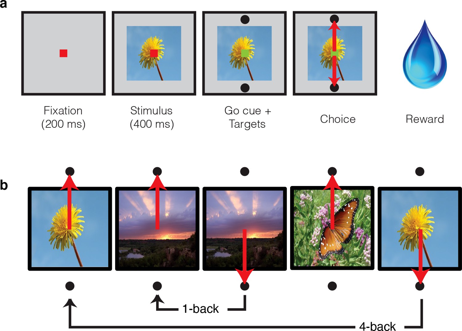
Single-exposure visual memory task.
In this task, monkeys viewed images and reported whether they were novel (i.e. had never been encountered before) or were familiar (had been encountered once and earlier in the same session) across a range of delays between novel and repeated presentations. (a) Each trial began with the monkey fixating for 200 ms. A stimulus was then shown for 400 ms, followed by a go cue, reflected by a change in the color of the fixation dot. Targets, located above and below the image, were associated with novel and familiar selections, and differed for each monkey. The image remained on the screen until a fixation break was detected. Successful completion of the trial resulted in a juice reward. (b) Example sequence where the upward target was associated with novel images, and the downward target with familiar images. Familiar images were presented with n-back of 1, 2, 4, 8, 16, 32, and 64 trials, corresponding to average delays of 4.5 s, 9 s, 18 s, 36 s, 1.2 min, 2.4 min, and 4.8 min, respectively. Additional representative images can be found in Figure 2—figure supplement 1.
Figure 2—figure supplement 1

Representative images used in the experiment, sampled from http://commons.wikimedia.org/wiki/Main_Page under the Creative Commons Attribution 4.0 International Public License https://creativecommons.org/licenses/by/4.0/.
https://doi.org/10.7554/eLife.32259.005
Figure 3
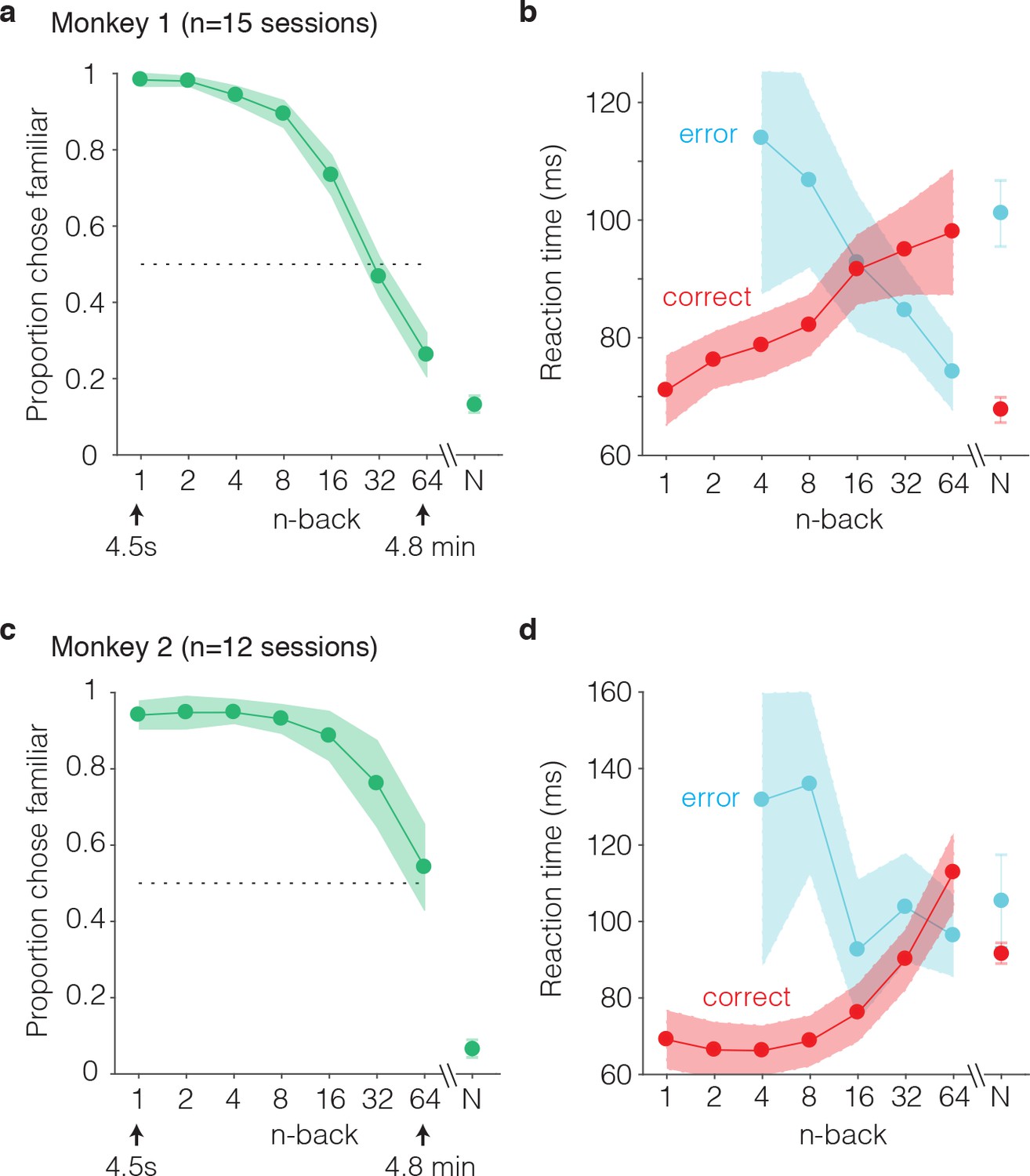
Behavioral performance of two monkeys on the single-trial visual recognition memory task.
(a,c) ‘Forgetting functions’, plotted as the proportion of trials that each monkey reported images as familiar as a function of the number of trials between novel and repeated presentations (n-back). Novel trials are indicated by ‘N’ and a break in the x-axis. The dotted line indicates chance performance on this task, 50%. Error bars depict 97.5% confidence intervals of the per-session means. (b,d) Mean reaction times, parsed according to trials in which the monkeys answered correctly versus made errors. Reaction times were measured relative to onset of the go cue, which was presented at 400 ms following stimulus onset. Error bars depict 97.5% confidence intervals computed across all trials.
Figure 4
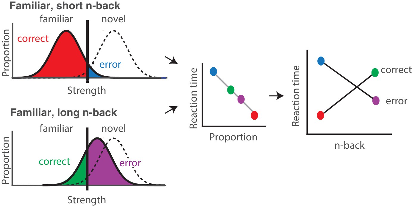
Strength theory qualitatively predicts x-shaped reaction time patterns.
Like signal detection theory, strength theory proposes that the value of a noisy internal variable, memory strength, is compared to a criterion to differentiate novel versus familiar predictions. Left: shown are the hypothetical distributions of memory strengths across a set of images presented as novel (dashed lines) and as familiar (black), repeated after a short (top) versus long (bottom) delay. The colored portions of each familiar distribution indicate the proportion of trials corresponding to correct reports and errors, based on the position of the distribution relative to the criterion. In the case of short n-back, memory strength is high, the proportion correct is high, and the proportion wrong is low. In the case of long n-back, memory strength is low, the proportion correct is low and the proportion wrong is high. Middle: strength theory proposes an inverted relationship between proportion and mean reaction times, depicted here as linear. Right: passing the distributions on the left through the linear function in the middle produces an x-shaped reaction time pattern.
Figure 5
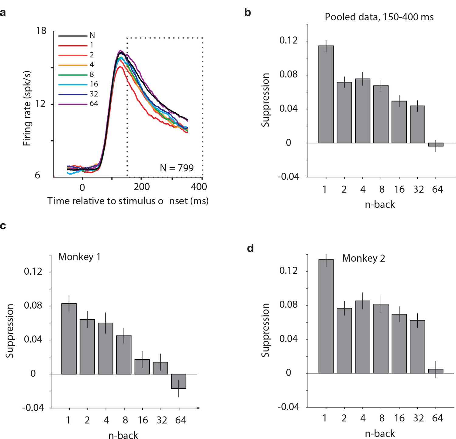
Average IT repetition suppression magnitudes.
(a) Grand mean firing rates for all units, plotted as a function of time aligned to stimulus onset, parsed by images presented as novel (black) versus familiar at different n-back (rainbow). Traces were computed in 1 ms bins and smoothed by averaging across 50 ms. The dotted box indicates the spike count window corresponding to the analysis presented in panels (b–d). The absence of data at the edges of the plot (−50:−25 ms and 375:400 ms) reflects that the data are plotted relative to the centers of each 50 ms bin and data were not analyzed before −50 ms or after the onset of the go cue at 400 ms. (b) The calculation of suppression magnitude at each n-back began by quantifying the grand mean firing rate response to novel and familiar images within a window positioned 150 ms to 400 ms after stimulus onset. Suppression magnitude was calculated separately for each n-back as (novel – familiar)/novel. (c–d) Suppression magnitudes at each n-back, computed as described for panel b but isolated to the units recorded in each monkey individually. Error reflects SEM.
Figure 6 with 1 supplement
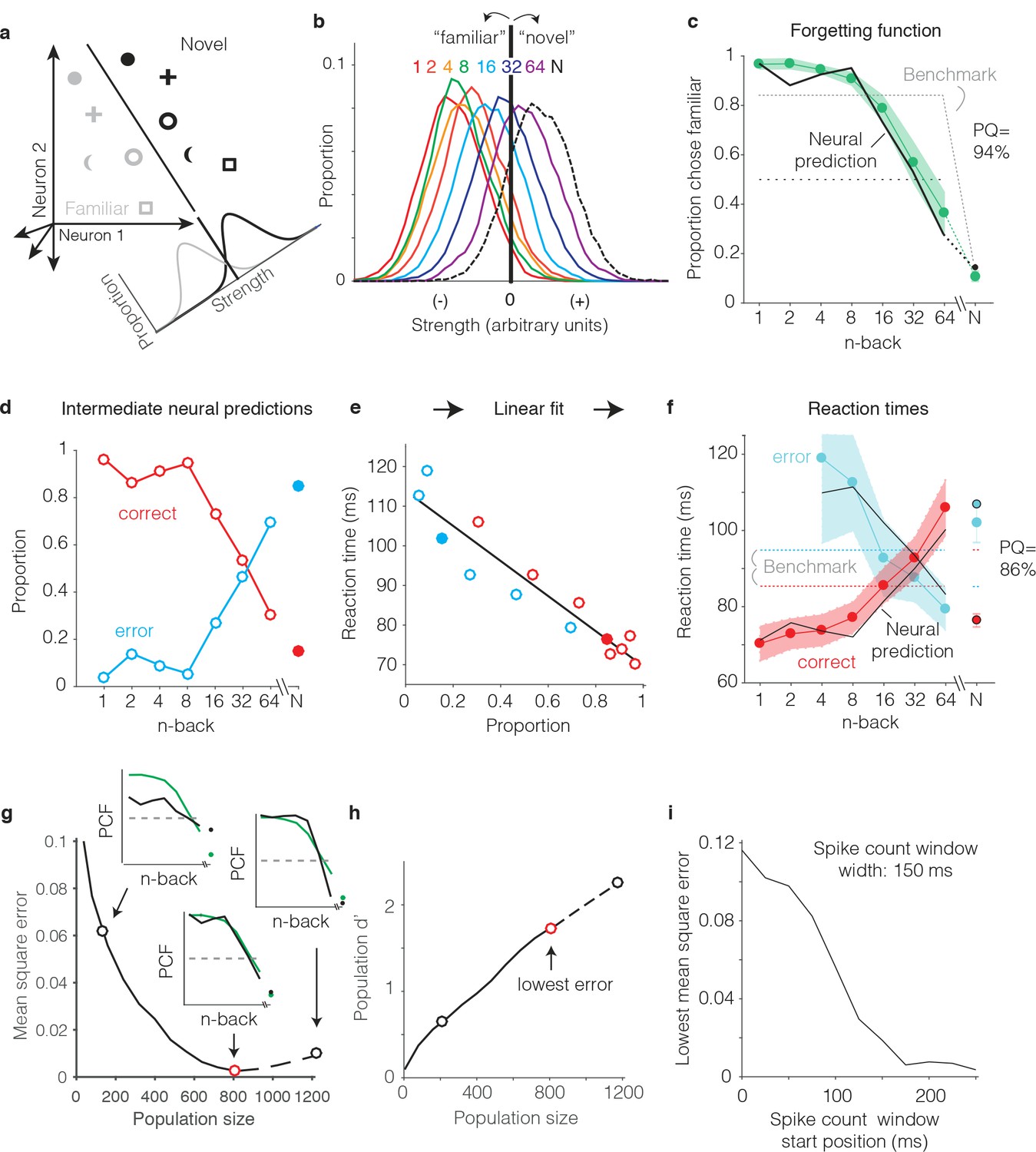
Transforming IT neural data into behavioral predictions.
In all panels, behavioral and neural data correspond to the data pooled across the two monkeys and methods are illustrated through application of only one linear decoder (the FLD). (a) A cartoon depiction of how memory strength was measured for each n-back. Shown are the hypothetical population responses of 2 neurons to different images (represented by different shapes) shown as novel (black) versus as familiar (gray). The line depicts a linear decoder decision boundary optimized to classify images as novel versus as familiar. Distributions across images within each class are calculated by computing the linearly weighted sum of each neuron’s responses and subtracting a criterion. (b) Distributions of the linearly weighted IT population response, as a measure of memory strength, shown for novel images (black dotted) and familiar images parsed by n-back (rainbow), for a population of 799 units. To compute these distributions, a linear decoder was trained to parse novel versus familiar across all n-back via an iterative resampling procedure (see Materials and methods). (c) Black: the neural prediction of the behavioral forgetting function, computed as the fraction of each distribution in panel b that fell on the ‘familiar’ (i.e. left) side of the criterion. Behavioral data are plotted with the same conventions as Figure 3a,c. Prediction quality (PQ) was measured relative to a step function benchmark (gray dotted) with matched average performance (see text). (d) The first step in the procedure for estimating reaction times, shown as a plot of the proportions of each distribution from panel b predicted to be correct versus wrong, as a function of n-back. Solid and open circles correspond to novel and familiar trials, respectively. Note that the red curve (correct trials) simply replots the predictions from panel c and the blue curve (error trials) simply depicts those same values, subtracted from 1. (e) A plot of the proportions plotted in panel d versus the monkeys’ mean reaction times for each condition, and a line fit to that data. (f) The final neural predictions for reaction times, computed by passing the data in panel d through the linear fit depicted in panel e. Behavioral data are plotted with the same conventions as Figure 3b,d. Also shown are the benchmarks used to compute PQ (labeled), computed by passing the benchmark values showing in panel c through the same process. (g) Mean squared error between the neural predictions of the forgetting function and the actual behavioral data, plotted as a function of population size. Solid lines correspond to the analysis applied to recorded data; the dashed line corresponds to the analysis applied to simulated extensions of the actual data (see Figure 6—figure supplement 1). Insets indicate examples of the alignment of the forgetting function and FLD neural prediction at three different population sizes, where green corresponds to the actual behavioral forgetting function and black corresponds to the neural prediction. PCF = proportion chose familiar. The red dot indicates the population size with the lowest error (n = 799 units). (h) Overall population d’ for the novel versus familiar task pooled across all n-back, plotted as a function of population size with the highlighted points from panel g indicated. (i) The analysis presented in panel g was repeated for spike count windows 150 ms wide shifted at different positions relative to stimulus onset. Shown is the minimal MSE for each window position. All other panels correspond to spikes counted 150–400 ms.
Figure 6—figure supplement 1
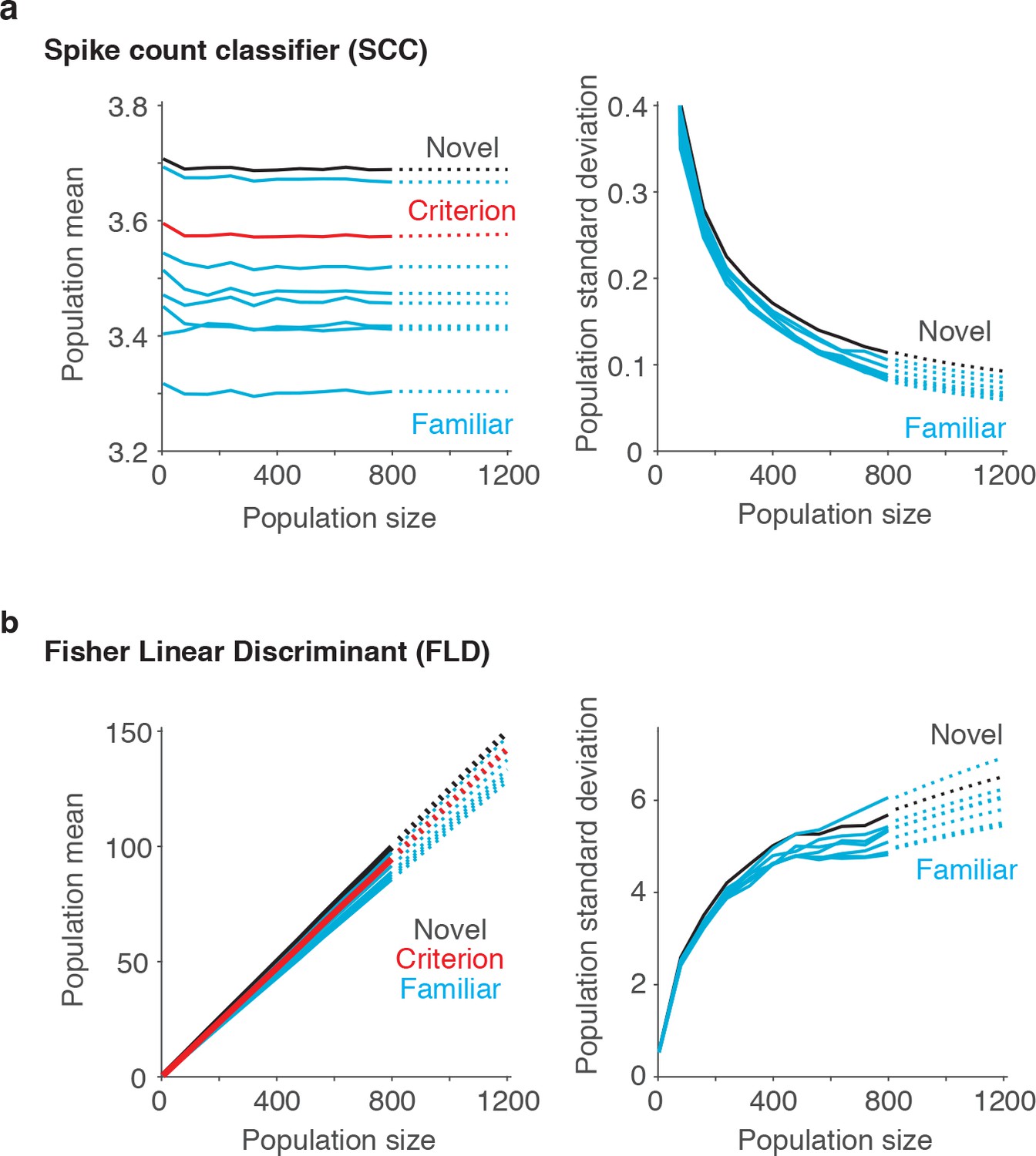
Extrapolating SCC and FLD predictions to larger sized populations.
To extrapolate neural predictions beyond the population sizes that we had recorded, we modeled the population response distributions at each n-back (Figure 6b) as Gaussian, and we estimated the means and standard deviations of each distribution at different population sizes by extending the trajectories computed from our data (solid lines) to estimates at larger population sizes (dotted lines). (a) In the case of the SCC, the mean population response was computed as the grand mean spike count across the population, and consequently did not grow with population size. We thus extended these trajectories with a simple linear fit to the values computed from the data. Shown are the population means computed for the novel images (black), the familiar images parsed by n-back (cyan) and the mean that corresponds to the criterion placement (red). In contrast, the standard deviations of these trajectories decreased as a function of population size and to extend these trajectories, we fit a two-parameter function (see Materials and methods). (b) In the case of the FLD, the population mean was computed as a weighted sum and grew linearly with population size. We extended these trajectories with a simple linear fit to the values computed from the data. In contrast, the FLD population standard deviation trajectories grew in a nonlinear manner, and to extend these trajectories, we fit a two-parameter function (see Materials and methods).
Figure 7 with 1 supplement
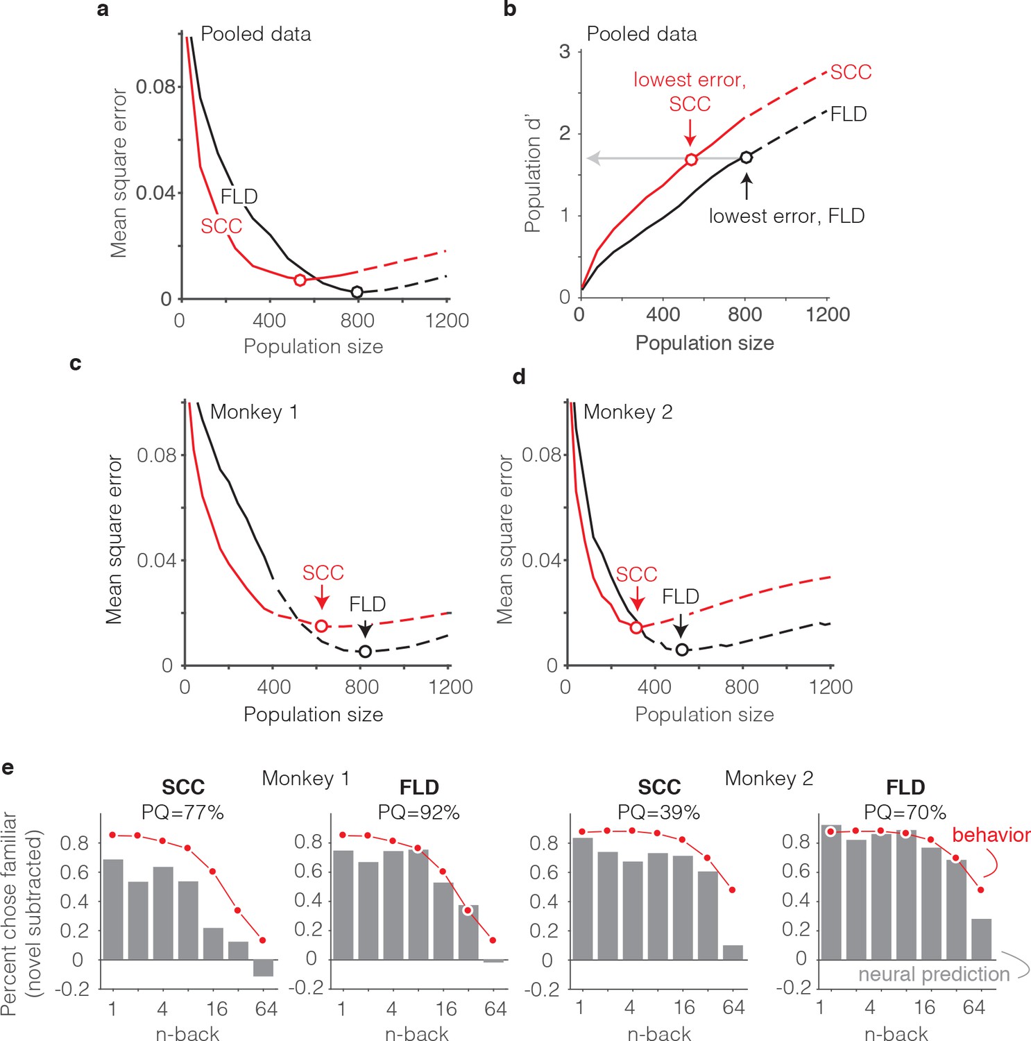
The FLD decoder is a better predictor of behavioral performance than the SCC.
(a) Plot of mean square error as a function of population size, computed as described for Figure 6g for the data pooled across both monkeys, and shown for both the FLD (black) and SCC (red) decoders. Dots correspond to the population size with the smallest error (FLD = 799 units; SCC = 625 units). (b) Plot of overall population d’ computed as described in Figure 6h but shown for both the FLD and SCC decoders. Dots correspond to the same (optimal) population sizes indicated in panel a. (c–d) The same analysis shown in panel a, but isolated to the data collected from each monkey individually. Best population sizes, Monkey 1: FLD = 800 units; SCC = 625 units; Monkey 2: FLD = 525 units; SCC = 316 units. (e) Gray: predicted forgetting functions, computed as described for Figure 6c, but plotted after subtracting the false alarm rate for novel images (i.e. a single value across all n-back). Red: the actual forgetting functions, also plotted after subtracting the novel image false alarm rate. These plots are a revisualization of the same data plotted before false alarm rate subtraction in Figure 7—figure supplement 1a-b. PQ: prediction quality, computed as described in panel 6 c.
Figure 7—figure supplement 1
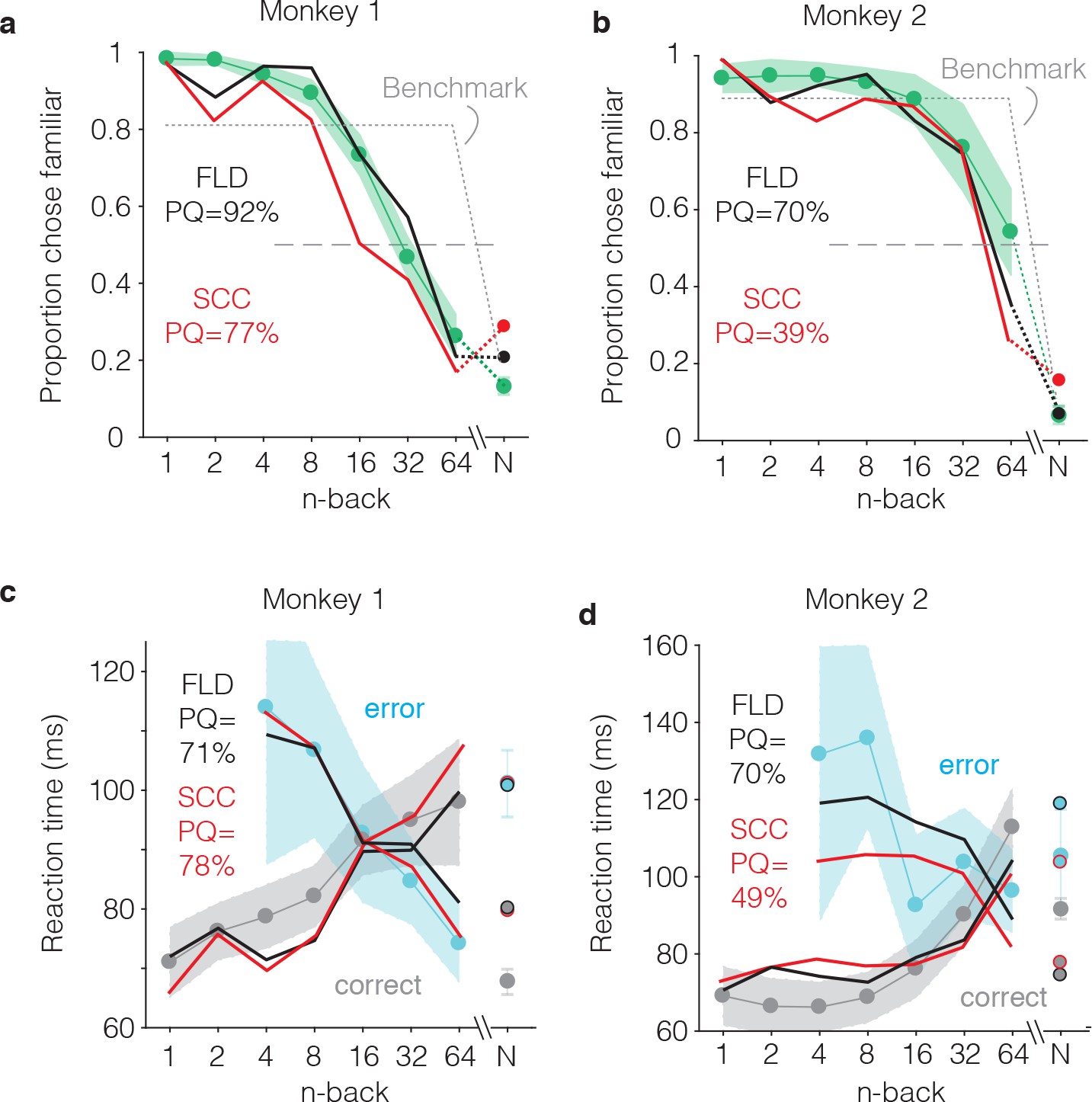
FLD and SCC predictions for each monkey.
(a–b) Predictions of the forgetting functions, computed as described for Figure 6c, but for both the SCC and FLD decoders and applied to the data from each monkey. (c–d) Predictions of reaction time patterns, computed as described for Figure 6f but for both the SCC and FLD decoders and applied to data from each monkey individually. To avoid clutter, the benchmark used to compute PQ is not shown. PQ: prediction quality. In both monkeys, the FLD predictions were generally well-aligned with reaction time patterns, including a x-shaped crossing point that corresponded to a higher n-back in the monkey that performed better at the task (monkey 2).
Figure 8
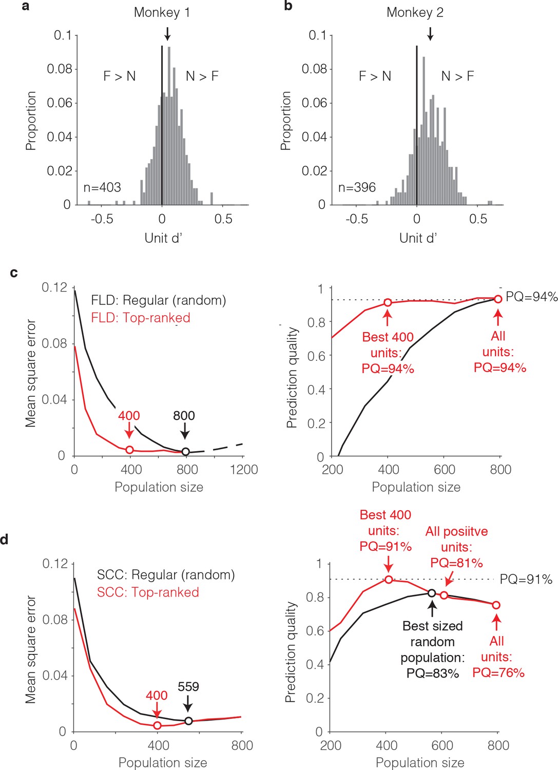
The single-unit correlates of the weighted linear decoding scheme.
(a–b) Distributions of unit d’, computed for each monkey. Arrows indicate means. (c) Left, Comparison of behavioral prediction error trajectories for an FLD decoder applied to randomly selected units (replotted from Figures 6g and 7a) versus when the top-ranked units for each population size were selected before cross-validated testing. Dots correspond to population sizes with lowest error. Right, Conversion of behavioral error predictions (MSE) into prediction quality (PQ). Dots indicate PQ for the best sized population and for all units. (d) Left, Comparison of behavioral prediction error trajectories for an SCC decoder applied to randomly selected units (replotted from Figure 7a) versus when the top-ranked units for each population size were selected before cross-validated testing. Dots correspond to population sizes with lowest error. Right, Conversion of MSE into PQ. Black dot indicates PQ for the best sized population for randomly selected units. Red dots indicate PQ for the 400 top-ranked, positive sign (d’>0) units, all positive sign units, and all units.
Figure 9
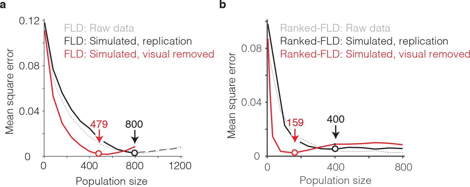
The impact of visual selectivity.
(a) FLD behavioral prediction error trajectories for the actual data (gray, replotted from Figure 6g), a simulated replication of the data in which both the visual selectivity and the visual memory signals for each unit were replicated (black), and a simulated version of the data in which the visual memory signals were preserved for each unit but visual selectivity was removed (see Materials and methods). (b) The same three FLD behavioral prediction error trajectories, computed with a ranked-FLD.
Figure 10
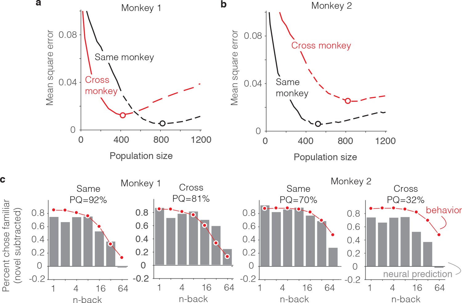
Alignment of individual behavioral and neural data.
(a–b) Plot of mean squared error as a function of population size, computed as described for Figure 6g but compared when behavioral and neural data come from the same monkey (black) versus when behavioral and neural data are crossed between monkeys (red). (c) Comparison of predicted and forgetting functions, plotted after subtracting the false alarm rate for novel images as in Figure 7e, for population sizes indicated by the dots in panels a-b. PQ = prediction quality.
Additional files
-
Source data 1
Data used to compare neural predictions with behavioral responses.
Behavioral data include the forgetting function and reaction times, each as a function of n-back. Neural data include the spike count responses of each unit to the same images presented as novel and as familiar at a range of n-back (Source_data.zip).
- https://doi.org/10.7554/eLife.32259.016
-
Transparent reporting form
- https://doi.org/10.7554/eLife.32259.017
Download links
A two-part list of links to download the article, or parts of the article, in various formats.
Downloads (link to download the article as PDF)
Open citations (links to open the citations from this article in various online reference manager services)
Cite this article (links to download the citations from this article in formats compatible with various reference manager tools)
Single-exposure visual memory judgments are reflected in inferotemporal cortex
eLife 7:e32259.
https://doi.org/10.7554/eLife.32259


