Structural and functional properties of a probabilistic model of neuronal connectivity in a simple locomotor network
- University of Plymouth, United Kingdom
- University of Bristol, United Kingdom
Figures
Figure 1
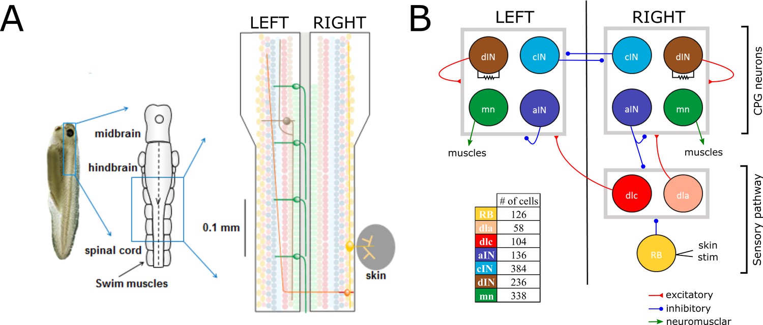
Swimming network.
(A) Left: Photo of a 5 mm long hatchling Xenopus tadpole. Middle: two-dimensional diagram showing the indicated region of CNS seen from top with its subdivisions (midbrain, hindbrain and spinal cord). Right: Zoom of the indicated region of hindbrain and rostral spinal cord after cutting the body in half along the midline and opening it like a book. The diagram shows examples of the position of cell bodies (filled circles), dendrites (straight horizontal lines) and axons (lines extending also vertically). The floor plate separates left and right side of the CNS (grey rectangle). (B) Diagram showing the different populations within the swimming network and the synaptic connections between them. Connections ending on the border of each symmetrical half-centres (grey square) represent connections to any cell-type in the corresponding half-center. Descending interneurons (dINs) are locally coupled by gap junctions. Note that neuronal populations in the sensory pathway are only shown for one side of the body, but are present on both sides in the model. The table shows the colour coding and the number of neurons for each neuron type.
Figure 2

Visualization of the probability matrix P.
(A) Image representation of the complete matrix , where the greyscale intensity of the pixel in row and column represents the value of the probability . Black intensity corresponds to connection probability zero and grey intensity close to white corresponds to connection probability one. Rows and columns corresponding to neurons of each of the seven types are separated by solid blue lines. These lines separate the matrix into symmetrical sub-blocks. Within each sub-block vertical and horizontal dotted lines separate the left body side (top rows and left columns) from the right body side (bottom rows and right columns). In each sub-block neurons are ordered according to increasing rostro-caudal position B. Zoom of the left body side aINaIN sub-block (marked by a red square in A).
Figure 3
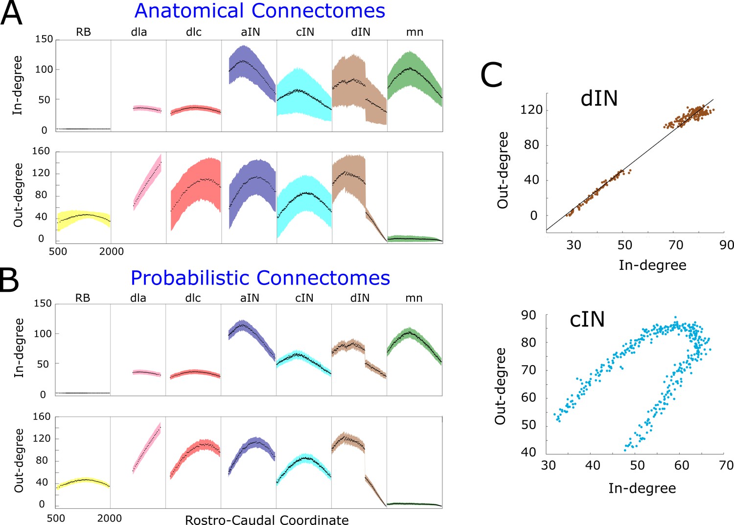
In- and out-degrees.
(A-B) Average in/out-degree and standard deviation for each cell in anatomical (A) and probabilistic (B) connectomes. Neurons are divided by cell type and their degrees are plotted as a function of their rostro-caudal (RC) position. (C) Scatter plots of in- vs out-degree for CPG neuron cINs and dINs (top) and cINs (bottom): light-blue and brown dots correspond to cIN and dIN neurons, respectively. Black line shows the linear regression model for dINs (r = 0.99).
Figure 4
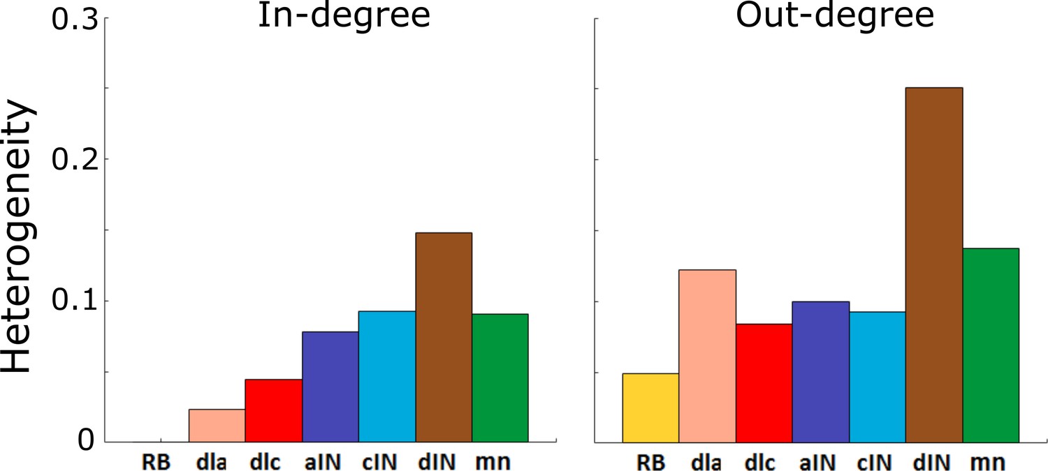
Heterogeneity index of the in-degree and out-degree distributions of each of the seven cell types.
https://doi.org/10.7554/eLife.33281.005
Figure 5
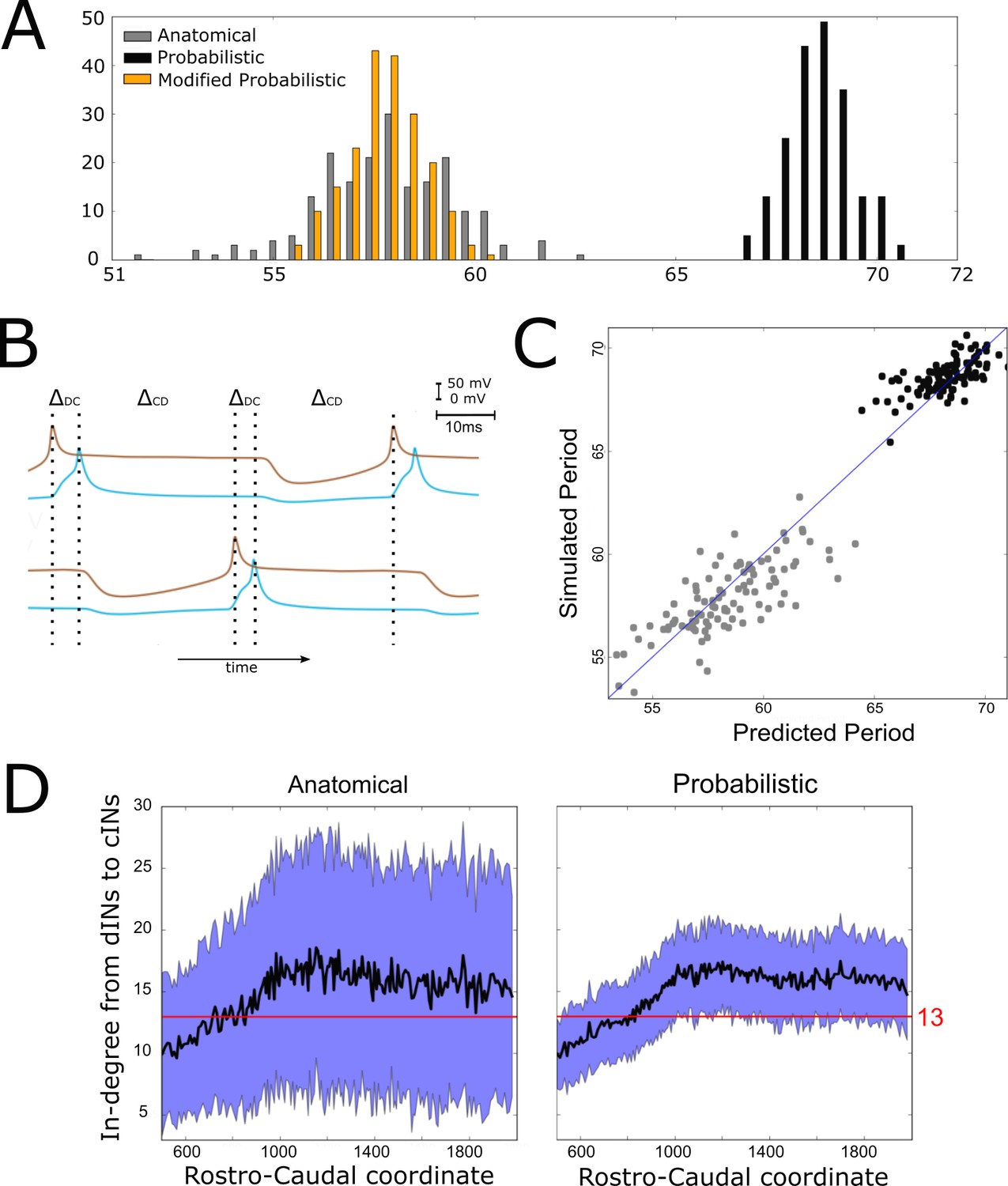
Investigating the difference in swimming cycle period between anatomical and probabilistic connectomes.
(A) Swimming period (as defined by median motoneuron spiking period) for 200 anatomical connectomes (grey), for 200 probabilistic connectomes (black) and 200 probabilistic connectomes where cIN to dIN synaptic strength is reduced (see text for details). (B) Example membrane potentials of example dINs (brown) and cINs (blue) on the left and right side during one swimming cycle. The swimming period is a sum of (twice) the delay between dIN and cIN spiking ( and (twice) the delay between cIN and contralateral dIN spiking (). (C) Network structure allows us to predict swimming period. Each point shows for one connectome (different from those used in part C and for linear regression) the predicted period based on the connectivity, with the actual period from simulation plotted on the vertical axis. The blue line shows the case where the prediction perfectly matches the simulation. (D) More cINs are inactive in anatomical connectomes than in probabilistic connectomes. Although the average in-degree (black line) is similar under both conditions, the standard deviation (blue area) is much higher for anatomical connectomes. This increased variance in anatomical connectomes means that more cINs receive fewer than the 13 connections from dINs that are required for reliable spiking.
Figure 6
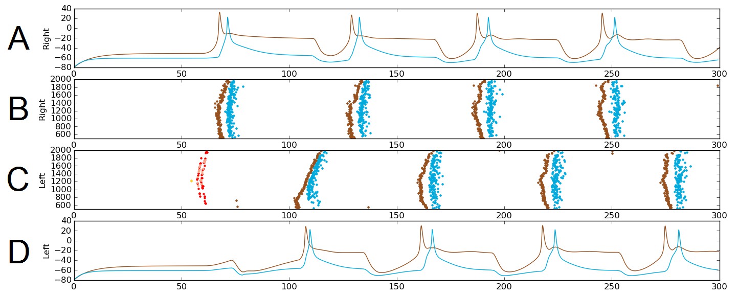
Alternating firing (‘swimming’) in one realization of the dIN-cIN subnetwork in a 300 ms simulation, showing activity on the right (A–B) and left (C–D) sides of the spinal cord.
B and C show spike times, where the vertical position of each spike corresponds to the rostro-caudal position of the associated neuron. A and D show voltage trace examples for single selected dINs (brown) and cINs (blue) on the right (A) and left (D). Simulated sensory stimulation at 50 ms causes an RB neuron (yellow) to spike, which excites dlas and dlcs (pink and red, respectively). Excitation from these sensory pathway neurons causes the dIN and cIN neurons that form the CPG to generate an alternating rhythm.
Figure 7
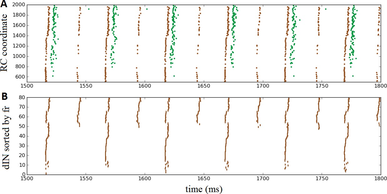
Oscillatory activity on one side of the body after removal of commissural connections.
(A) Raster plot of spiking activity during swimming, showing dINs (brown) and motoneurons (green) on the left side of the spinal cord after removal of commissural connections. (B) The same dIN spiking activity as in (A), but with the spike trains sorted vertically based on increasing firing rate. In both cases, activity is shown between 1500 and 1800 ms post-stimulation, when the system has settled down into a stable oscillatory state.
Figure 8
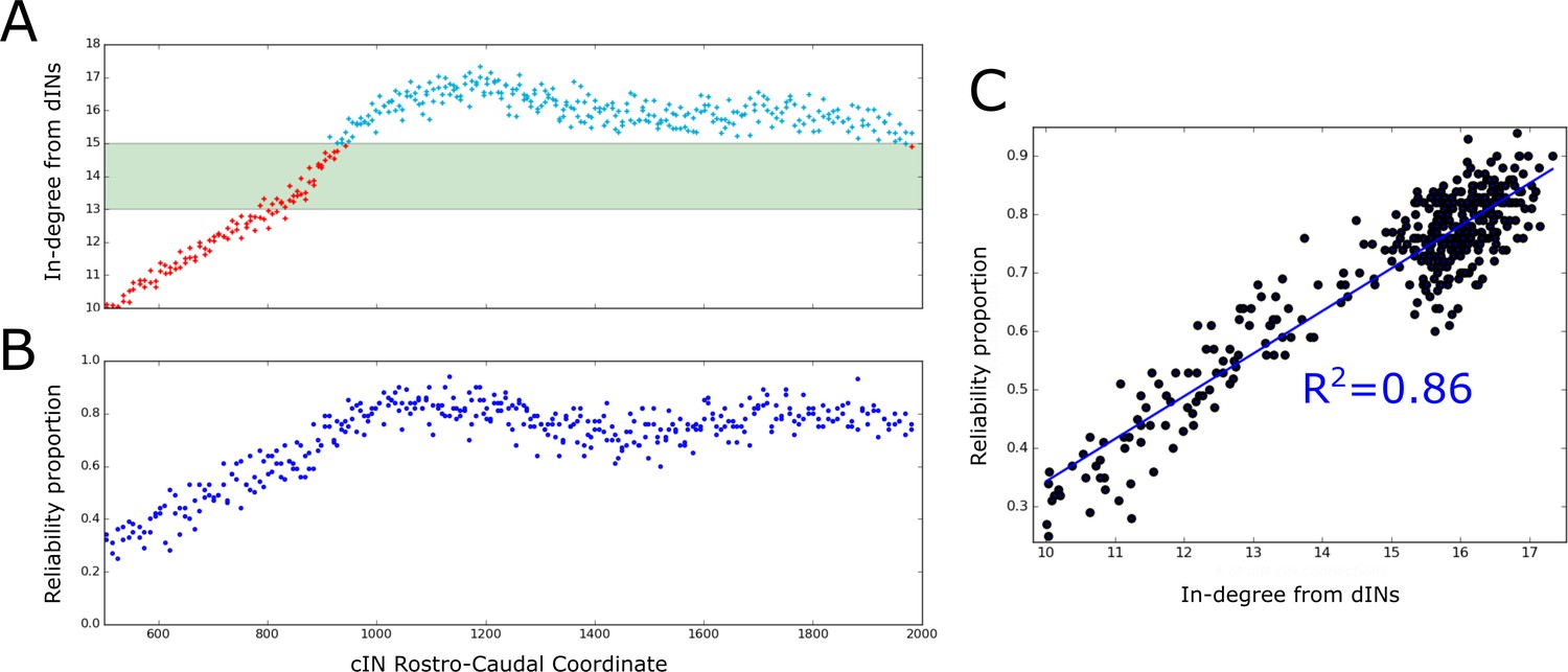
Firing reliability of cINs.
(A) Plot of the average cIN in-degree from pre-synaptic dINs as a function of rostro-caudal position. Blue dots represent cINs that have on average 15 or more incoming connections from dINs, while red dots represent cINs that have on average fewer than 15 incoming connections from dINs. The cINs with 13–15 incoming connections (green shaded area) are most likely to fire unreliably, whereas those with fewer than 13 connections are likely to be completely inactive. (B) cIN reliability proportion vs cIN rostro-caudal position; for each cIN the reliability proportion is the fraction of 100 simulations where the cIN fires reliably. (C) Scatter plot of the cIN reliability proportion vs the average in-degree from dINs. The figure shows the linear regression line between these two variables and the corresponding value.
Figure 9
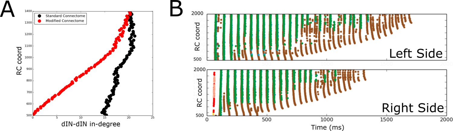
Comparison of spiking activity in the normal case and when dIN ascending axons are removed.
(A) Average in-degree from dINs to other dINs at different rostro-caudal positions in the standard connectome (black dots) and after removal of ascending dIN axons (red dots). (B) Example of typical spiking activities from connectomes with ascending dIN axons removed (case 1, see text for details).
Tables
Appendix 2—table 1
Maximal conductance (in nS) and equilibrium potential (in mV) of each ionic channel in the model neurons.
https://doi.org/10.7554/eLife.33281.014| dIN | 1.4 | −52 | 240.5 | 50 | 12 | −80 | 9.6 | −80 |
| non−dIN | 2.47 | −61 | 110 | 50 | 8 | −80 | 1 | −80 |
Appendix 2—table 2
Parameters defining the rate functions of the model neurons rounded to the first decimal digit for dINs and non-dIN neuronal types ( sign that the cell type has no contribution of the specific channel variable, units of measures are given in the first row of each parameter; parameter is dimensionless).
https://doi.org/10.7554/eLife.33281.015| dIN / non−dlN | Rate Function | A (ms -1) | B (ms−1mV−1) | C (−) | D (mV) | E (mV) |
|---|---|---|---|---|---|---|
| Ca | 4/− | 0/− | 1/− | −15.3/− | −13.6/− | |
| 1.2/− | 0/− | 1/− | 10.6/− | 1/− | ||
| 1.3/− | 0/− | 1/− | 5.4/− | 12.1/− | ||
| K−fast | 5.1/3.1 | 0.1/0 | 5.1/1 | −18.4/−27.5 | −25.4/−9.3 | |
| 0.5/0.4 | 0/0 | 0/1 | 28.7/9 | 34.6/16.2 | ||
| K−slow | 0.5/0.2 | 8.2e − 3/0 | 4.6/1 | −4.2/−3 | −12/−7.7 | |
| 0.1/0.05 | −1.3e − 3/0 | 1.6/1 | 2.1e5/−14.1 | 3.3e5/6.1 | ||
| Na | 8.7/13.3 | 0/0 | 1/0.5 | −1/−5. | 12.6/−12.6 | |
| 3.8/5.7 | 0/0 | 1/1 | 9/5 | 9.7/9.7 | ||
| 0.1/0.04 | 0/0 | 0/0 | 38.9/28.8 | 26/26 | ||
| 4.1/2 | 0/0 | 1/1e−3 | −5.1/−9.1 | −10.2/−10.2 |
Appendix 2—table 3
Parameters of the synaptic models.
https://doi.org/10.7554/eLife.33281.016| X | NMDA | AMPA | INH |
|---|---|---|---|
| 0.5 | 0.2 | 1.5 | |
| 80 | 3.0 | 4.0 | |
| 1.25 | 1.25 | 3.0 | |
| 0 | 0 | −75 | |
| 0.29 | 0.593 | 0.435 |
Additional files
-
Transparent reporting form
- https://doi.org/10.7554/eLife.33281.011
Download links
A two-part list of links to download the article, or parts of the article, in various formats.
Downloads (link to download the article as PDF)
Open citations (links to open the citations from this article in various online reference manager services)
Cite this article (links to download the citations from this article in formats compatible with various reference manager tools)
Structural and functional properties of a probabilistic model of neuronal connectivity in a simple locomotor network
eLife 7:e33281.
https://doi.org/10.7554/eLife.33281


