Inferring circuit mechanisms from sparse neural recording and global perturbation in grid cells
- The University of California, United States
- The University of Texas, United States
Figures
Figure 1 with 2 supplements
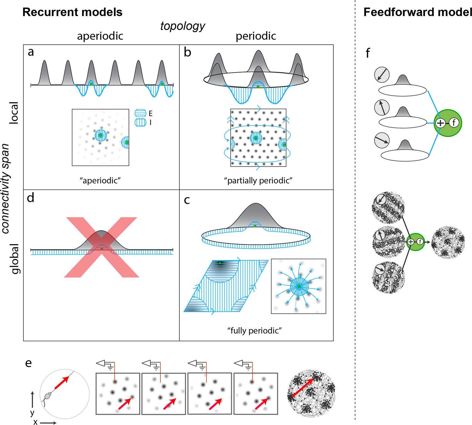
Mechanistically distinct models that cannot be ruled out with existing results.
(a–d) Recurrent pattern-forming models. Gray bumps: population activity profiles. Blue: Profile of synaptic weights from a representative grid cell (green) to the rest of the network. Bottom of each panel: 2D network; Top: equivalent 1D toy network. Matching arrows along a pair of straight network edges signify that those edges are glued together. (a) Aperiodic network: (Burak and Fiete, 2009; Widloski and Fiete, 2014): local connectivity without periodic network boundaries. (b) Partially periodic network (Burak and Fiete, 2009): local connectivity in a network with periodic boundaries. (c) Bottom left and top: Fully periodic network (Guanella et al., 2007; Burak and Fiete, 2006; Fuhs and Touretzky, 2006; Pastoll et al., 2013; Brecht et al., 2014; Widloski and Fiete, 2014), with global connectivity and periodic boundaries. Bottom right: multi-bump network with local-looking connectivity but long-range connections between co-active cells in different bumps. This model is mathematically equivalent to a fully periodic model (see Figure 1—figure supplement 1). (d) A network with a single activity bump and without periodic boundaries cannot properly retain phase information as the bump moves around: it will not be a good integrator of animal velocity and is not a candidate mechanism. (e) Movement of the animal (left) causes a flow of the population pattern in proportion to animal velocity (four snapshots over time in center panels) for the models in (a–c). Red line: Electrode whose tip marks the location of a recorded cell. The recorded cell’s response is spatially periodic (right; spikes in black), like grid cells. (f) Feedforward model: A grid cell (green) receives and combines inputs that are spatially tuned with uniform resolution across open spaces (implying these inputs reflect path integration-baed location estimates). These inputs may arise from recurrent ring attractor networks (Mhatre et al., 2012; Blair et al., 2008) (top) and exhibit stripe-like spatial tuning either in their firing rates (Mhatre et al., 2012) (bottom left) or firing phase with respect to the theta-band LFP oscillation (Welday et al., 2011; Bush and Burgess, 2014) (not shown). Or, they could arise from place cells assumed to path integrate (Kropff and Treves, 2008; Dordek et al., 2016). Selective feedforward summation followed by a nonlinearity produces grid-like responses (bottom right).
Figure 1—figure supplement 1

(Weakly) coupling neurons based on periodic activity patterning converts an aperiodic network into an effectively fully periodic one.
(a) The population pattern period in an aperiodic network expands continuously with increasing inhibition strength () over a range. The ordinate shows the stretch-factor , which quantifies the deviation of the period post-perturbation from that pre-perturbation, normalized by the pre-perturbation period (see Materials and methods). Altering the network’s connectivity to even slightly take into account the periodic activity pattern by adding weak connections between neurons in adjacent activity bumps (as in [b]) transforms the network into one that will not stretch at all (cyan curve). This network with coupled activity bumps, despite the weakness of the connectivity, is in principle mathematically analogous to the fully periodic network. Indeed, the population period in the network with cyan connectivity can no longer gradually vary with inhibition strength (cyan curve, (a)). Simulation details: The network connectivity is a hybrid of the aperiodic network in Burak and Fiete, 2009 with the fully periodic network of Fuhs and Touretzky, 2006 (note that, while the model of Fuhs and Touretzky, 2006 does not have explicit periodic boundary conditions, the multimodality of the synaptic weights couples adjacent activity bumps so that the network acts as a single-bump, fully periodic network). The dynamics are LNP-based (see Materials and methods) and driven with inputs simulating animal motion at constant speed (v = 0.3 m/s) for 10 s. There are only two populations (call them R and L), distinct in their directional preferences ( (0,1), (0,–1) for the R and L populations, respectively) and output synaptic asymmetries (see below). The shifted output weight profiles are sinusoids with gaussian envelopes, the latter which constrain the non-locality of the projections. For a narrow gaussian envelope, the weights resemble the purely local, center-surround profiles of Burak and Fiete, 2009, whereas for wide gaussian envelopes, the weights resemble the non-local, multimodal projections of Fuhs and Touretzky, 2006. The weights going from population to and from cells i and j, are given by , where ( for and ), is a scaling factor that modulates the amplitude of the weights, is a normalization factor, determines the width of the gaussian envelope, and determines the period of the underlying sinusoid. Parameters. 200 neurons; CV = 0.5; 0.5 ms; 30 ms; 50; 0; 1; ; ; = 200; 412.
Figure 1—figure supplement 2
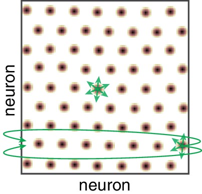
The a priori theoretical implausibility of partially periodic networks.
Population activity in the cortical sheet (yellow-black blobs), with schematic of connectivity (green). Note that in the bulk of the sheet, connectivity is local and not determined by the periodic activity in the sheet. However, the imposition of periodic boundary conditions requires that some neurons connect with others on the far edge of the sheet. Even if neurons are not topographically organized, the connectivity requires that a planar cortical sheet is somehow intrinsically connected as a torus. Activity-dependent weight changes that are based on the expression of periodic activity patterns could produce a torus-like connectivity, but then if the sheet is not topographically ordered it is likely that neurons in various bumps will connect to each other, producing a fully periodic rather than partially periodic network.
Figure 2 with 4 supplements
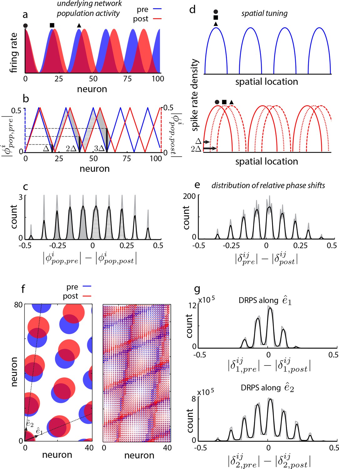
Global perturbation with analysis of phase shifts: signatures of recurrent patterning.
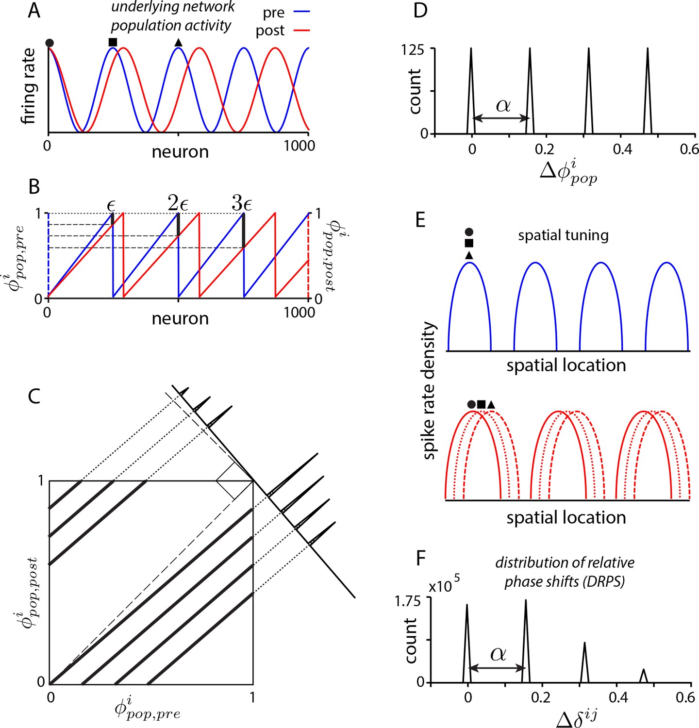
(a) Schematic of population activity before (blue) and after (red) a 10% period expansion (; the center of expansion is shown at left, but results are independent of this choice) in an aperiodic network. Circle, square, triangle: three sample cells with the same pre-expansion population phase. (b) The population phase of the th neuron is defined as where is the population pattern period. Plotted: population phase magnitudes pre- (blue) and post- (red) expansion (phase magnitude is given by the Lee distance, , where denotes absolute value). (c) Histogram of quantal shifts in the pre-to post-expansion population phases for all (n = 100) cells in the network. Gray line: raw histogram (200 bins). Black line: smoothed histogram (convolution with 2-bin Gaussian). Negative (positive) phase shifts arise from gray-shaded (horizontally-striped) areas in (b). (d–e) Quantal shifts in the population phase (experimentally inaccessible) are mirrored in shifts in the pairwise relative phase of spatial tuning between cells (experimentally observable). (d) Schematic of spatial tuning curves of three cells (circle, square, triangle) from (a). Pre-expansion the tuning curves have the same phase (top), thus their relative spatial tuning phases are zero. The tuning curves become offset post-expansion (bottom), because the shift in the population pattern forces them to stop being coactive. (e) Distribution of relative phase shifts (DRPS; gray). Relative phase between cells ( is the offset of the central peak in the cross-correlation of their spatial tuning curves; is their shared spatial tuning period). A relative phase shift is the difference in relative phase between a pair of cells pre- to post-perturbation. Black: smoothed version. There are (100 choose 2)=4950 pairwise relative phase samples. (f) Population activity pattern and pattern phase pre- and post-expansion in a 2D grid network (as in (a–b)). Dotted lines: principal axes of the population pattern (left). An arrow marks each cell’s population phase (right). (g) DRPS for the two components of 2D relative phase (as in (e); see Materials and methods). Samples: (3200 choose 2).
Figure 2—figure supplement 1
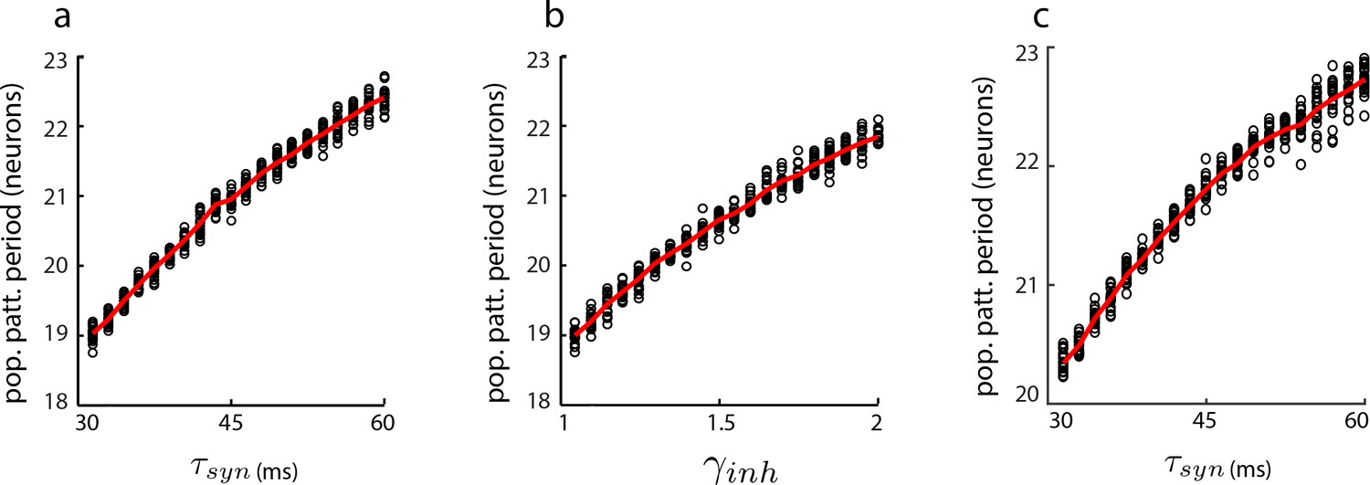
Dynamical simulations of the aperiodic network with LNP dynamics: gradual change in population period.
Change in population pattern period as the the time-constant (a) and inhibition strength (b) are increased in a 1D aperiodic network (see Materials and methods). In all trials (black circles), the network is driven by a constant velocity input (v = 0.3 m/s) for 10 s. Red line: average (n = 50 for each parameter value). In (c), same as in (a), except that velocity input into each neuron is additive instead of multiplicative (see Materials and methods).
Figure 2—figure supplement 2
When the 2:1 relationship between number of peaks in the DRPS and the number of bumps in the population pattern breaks down.
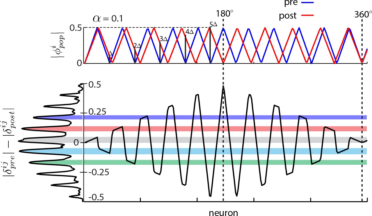
Top: Schematic of the phase in a population pattern, pre- (blue) and post- (red) perturbation, for a large 1D network with many bumps with population period stretch factor =0.1, with phase shift quanta indicated by black vertical bars for cells lying at integer multiples of the pre-perturbation wavelength. Bottom: Black curve: Difference in the pre- and post-perturbation phases of cells. At left, the DRPS is aligned vertically with the y-axis of the phase shift plot, so that the origin of the DRPS peaks is more readily apparent. For the neuron lying one wavelength away from the center of expansion, we define its phase shift as one ‘quantum’, . is related to the stretch factor via . The peak locations in the DRPS at bottom left correspond roughly to all half integer multiples of . After moving five bumps away from the center of expansion, the phase shift has reached its maximum at 0.5. At this point, there can be no additional (farther out) quantal peaks in the DRPS, meaning that only patterns of up bumps can be discriminated. Thus, the number of DRPS peaks equals twice the number of bumps, , in the pattern only when ; when , the number of peaks in the DRPS will systematically underestimate the number of bumps in the pattern.
Figure 2—figure supplement 3
Alternative formulation of the DRPS.
(a) 1D population activity, pre- (blue) and post-perturbation, for a increase the wavelength of the pattern ( neurons), with pattern expansion is centered at the left network edge. Circle, square, and triangle: locations of cells that are separated by integer numbers of wavelengths. (b) Population phase, pre- (blue) and post- (red) perturbation (see Materials and methods subsection ‘Alternative formulation of the DRPS’ for definitions and transformations in this context). (c) Post-perturbation phase vs. pre-perturbation phase, with projection of data onto orthogonal axis shown at upper right (see Materials and methods). (d) Distribution of shifts in population phase (n = 1000) (see Materials and methods). (e–f) Shift distributions for population phase (experimentally inaccessible) carry over to shift distributions for spatial tuning phase (experimentally observable). (e) The circle, square, and triangle cells, which original have identical spatial tuning (blue curves), now exhibit shifted spatial tuning curves (red curves). The shift in spatial phase for a pair is proportional to the number of activity bumps between them in the original population activity pattern. (f) Distribution of relative phase shifts (DRPS) ( (1000 choose 2) relative phase samples because relative phase is computed pairwise) (see Materials and methods).
Figure 2—figure supplement 4
Cortical Hodgkin-Huxley (CHH) simulations to assess the effects of cooling as an experimental perturbation and to elucidate the link between temperature and parameter settings in grid cell models with simpler neurons.
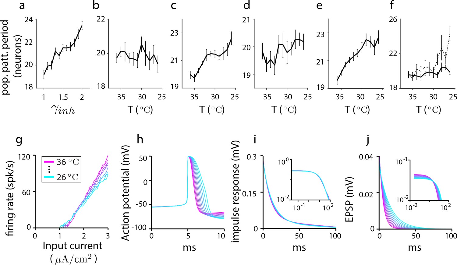
Results from a 1D aperiodic recurrent network grid cell model with CHH neurons. In all simulations, the network is driven by a constant velocity of 0.3 m/s and the run is a 10 s trajectory. (a–d) The change in population period as parameters are varied to simulate thermal and neuromodulatory effects (see Materials and methods). (a) Population period increases gradually with the strength of inhibition. Each point is the population period averaged over 10 trials (error bars reflect the SEM). (b) Effect of temperature on period through ionic conductances: Only the ionic parameters (and not the synaptic parameters) are varied according to their factors (see Materials and methods). The population period shrinks with decreasing temperature. (c) Effect of temperature on period through synaptic parameters: Temperature perturbation of only the synaptic parameters (and not the ionic parameters) causes the population period to expand with decreasing temperature. (d) Total effect of temperature on period through all ionic and synaptic parameters: All synaptic and ionic parameters are varied according to their factors (see Materials and methods) as temperature is stepped down from C to C. The combined effect is an increase in population period with decreasing temperature. Thus, we may predict that the effect of cooling the experimental system should be an expansion of the population period. We conclude from (b–d) that synaptic parameter changes trump the opposing effects of ionic versus synaptic temperature-dependent changes on population period. We also conclude that, because synaptic effects dominate over cellular effects, we may reasonably mimic the effects of temperature in network simulations with simpler neurons by using the synaptic model of the CHH simulations together with the prescribed temperature-dependent modification of synaptic parameters, while neglecting how temperature might affect neural parameters and equations (e) Dissecting synaptic temperature effects: Temperature modulation of only the synaptic time constant, leaving synaptic conductances unchanged. (f) Dissecting synaptic temperature effects: Temperature modulation of only the synaptic conductances, leaving the synaptic time constants unchanged (solid line). The effect on period of conductance modulation is weaker than the effect of time constant modulation. (This difference can be traced to the larger modulation of the time-constant: If the factor for synaptic conductances is set to be that of the time constant (dotted line), the effects on population period become comparable; compare with (e)). Summarizing (b–f), ionic and synaptic temperature modulations have opposing effects on period, but synaptic effects dominate leading to an increase in period with decreasing period. Within synaptic parameters, time constant effects on period dominate over conductance effects. Thus, in simpler neuron models of grid cells, the effect of temperature can be roughly approximated by scaling without a rescaling of the other parameters. (g–j) How temperature changes single-cell and synaptic properties in CHH models when all synaptic and ionic parameters are changed according to their respective factors. (g) Firing rate as a function of input current, (h) action potential shape, and (i) impulse response (i.e., subthreshold response of membrane potential to current pulse), with log-log plot in inset. (j) The net EPSP shape as a function of temperature. There is a slight decrease in the overall amplitude of the EPSP with temperature (as shown by the log-log plot of the same data in the inset), but this change is small compared to the effect on the EPSP time constant, consistent with (e–f).
Figure 3 with 1 supplement
Effects of perturbation in recurrent and feedforward neural network simulations: predictions for experiment.
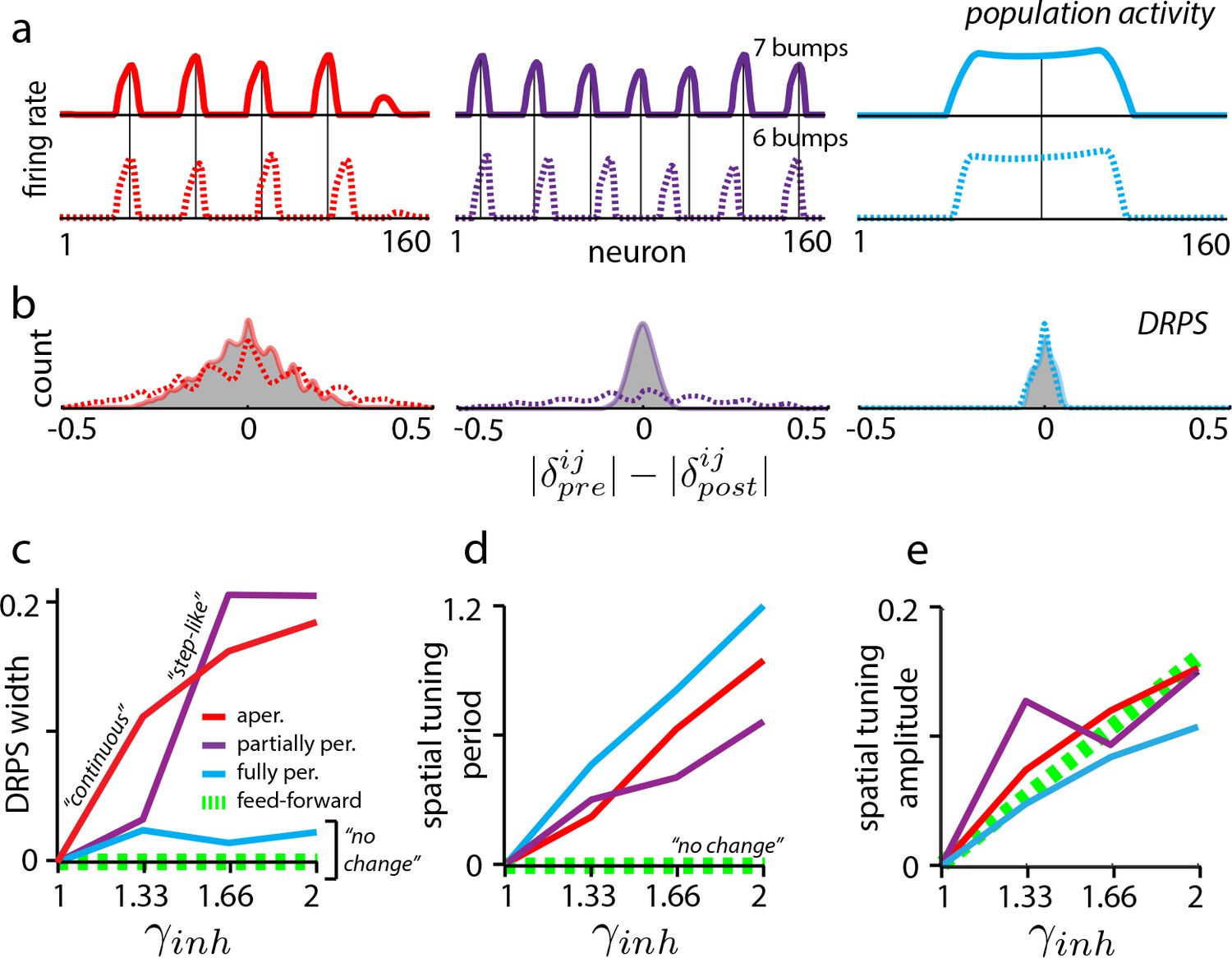
(a) Simulations of aperiodic (column 1), partially periodic (column 2), and fully periodic (column 3) networks show changes in the population pattern pre-perturbation (first row; ) to post-perturbation (second row; ). Solid vertical lines: pre-perturbation bump locations. (Simulation details in Materials and methods.) (b) Perturbation-induced DRPS in the various networks for two perturbation strengths (: solid line and filled gray area; : dotted line), both relative to the unperturbed case. (c) DRPS width (, defined as the standard deviation of the DRPS) as a function of perturbation strength for the different networks. Dashed green line: feedforward networks (predicted, not from simulation). The step-like shape for the partially periodic network is generic; however, the point at which the step occurs may vary from trial to trial. (d–e) Change in spatial tuning period (d) and amplitude (e) as a function of the perturbation strength (see Materials and methods). Change is defined as , where is the spatial tuning period or amplitude.
Figure 3—figure supplement 1
Changes in spatial tuning period in neural network simulations of the grid cell circuit are due to changes in both the population period and the velocity response of the network.
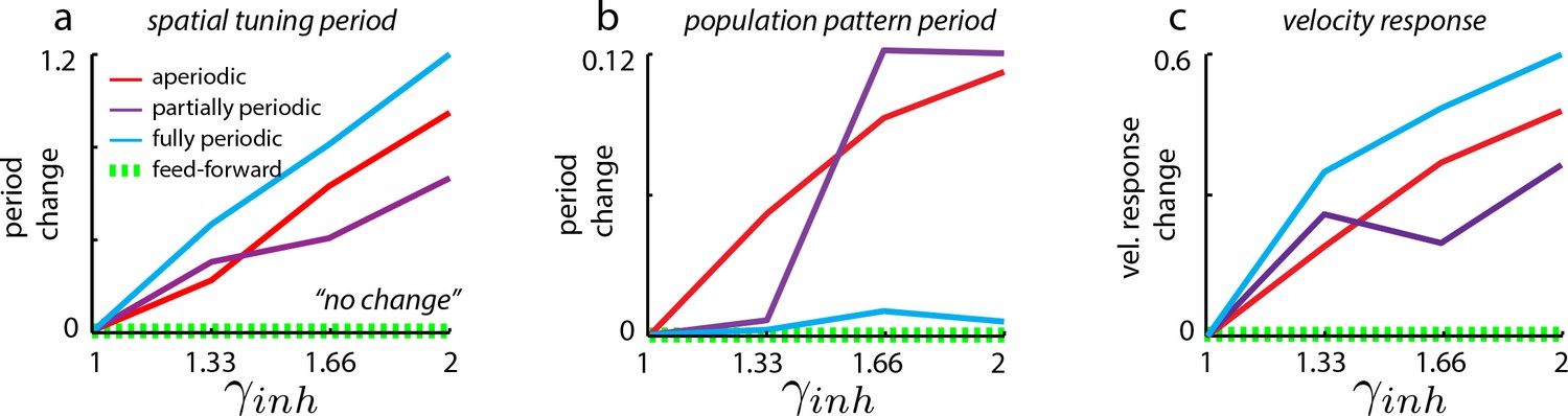
Change in spatial tuning period (a), population pattern period (b), and the velocity response (c) for the different network architectures (see Materials and methods for definitions of measures). Change is defined for quantity as , where refers to that quantity measured in the unperturbed () case, and refers to that quantity as measured in the perturbed (=1.33, 1.66, 2) cases. It is clear that the spatial tuning period (a) is more strongly influenced by the velocity response (c) than by the population period (b).
Figure 4 with 1 supplement
Data limitations and the resolvability of predictions.
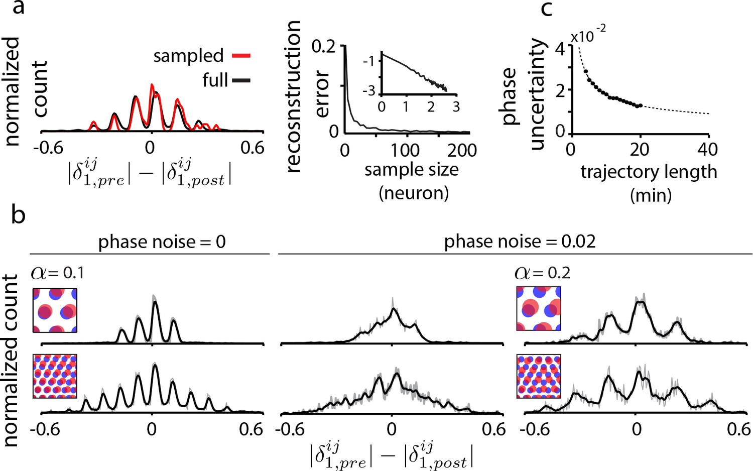
(a) Left: The quantal structure of the DRPS (along first principal axis of the 2D phase) is apparent even in small samples of the population (black: full population; red: n = 10 cells out of 1600; stretch factor ). Right: The L2-norm difference between the full and sampled DRPS as a function of number of sampled cells. Inset: log-log scale. (b) First and second rows: DRPS for population patterns with different numbers of bumps (gray line: raw; black line: smoothed with 2-bin Gaussian). Column 1: zero error or noise in estimating relative phase. Column 2: same DRPS’ as in column 1, but with phase estimation errors (i.i.d. additive Gaussian noise with zero mean and standard deviation 0.02 for each component of the relative phase vector, ). Column 3: Increasing the stretch factor () renders the peaks in the DRPS more discernible at a fixed level of phase noise. For the 5-bump pattern (second row), and thus the number of peaks in the DRPS times 1/2 at this larger stretch factor will underestimate the number of bumps in the underlying population pattern. (c) In grid cell recordings (data from Hafting et al., 2005), the uncertainty in measuring relative phase, as estimated by bootstrap sampling from the full dataset (see Materials and methods), declines with the length of the data record according to (dotted line). Parameters: neurons (a) =20 neurons (b, top row),=8 neurons (b, bottom row); = 0.1; ; network size: neurons.
Figure 4—figure supplement 1
Effects of uncertainty in phase estimation.
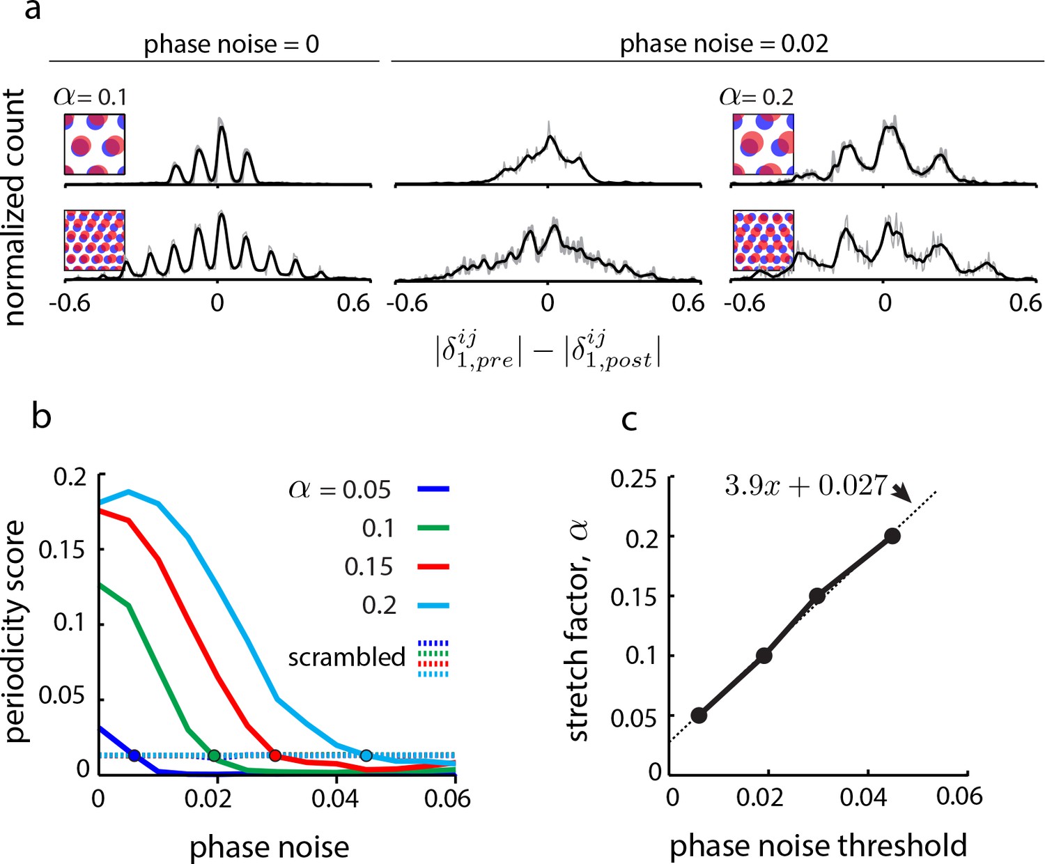
(a) Copied from Figure 4b. First and second columns: DRPS (200 bins; gray line: raw; black line: smoothed with 2-bin Gaussian) for different numbers of population pattern bumps along the first principal axis of the pattern and for different amounts of phase noise (noise is sampled i.i.d. from a gaussian distribution, , and added to each component of the relative phase vector, ; ‘phase noise’ is the same as ). Third column: Same as the second column, except for a larger stretch factor, . Note that the peak separation has increased so that the individual peaks are discernible. However, for the five bump network in the second row, inferring the number of bumps in the underlying population pattern would lead to an underestimate, since . (b) Solid lines: Periodicity score (a measure of how well separated and equidistant are the peaks in the DRPS, and ranges between 0 and 1; see Materials and methods) as a function of phase noise for 2-bump network in (a), for different values of the stretch factor, (solid lines). Periodicity is measured for the DRPS along the first principal axis. Dashed lines: Same as solid lines, except computed by randomly shuffling the phase vectors post-perturbation. (c) Stretch factor, , as a function of threshold phase noise (defined as the phase noise where the DRPS is indistinguishable from the DRPS when the phase vectors in the post-perturbation condition are reassigned randomly, i.e., the value of the phase noise when the colored curves in (b) cross the respective colored dashed lines).
Figure 5 with 5 supplements
Decision tree for experimentally discriminating circuit mechanisms.
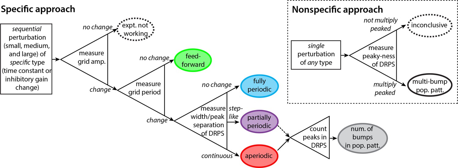
The ‘specific’ approach involves a specific perturbation to either the gain of inhibition or the neural time-constants. Under the assumption of this kind of perturbation, the period, the amplitude, and the relative phases of the spatial tuning curves of neurons are measured pre-perturbation and then for each of three increasingly strong perturbations. A change in spatial tuning amplitude means that the attempted perturbation is in effect. Recurrent mechanisms can be discriminated from feedforward ones based on whether the perturbation changes the spatial tuning period (first open triangle). Different recurrent networks can be discriminated from each other based on the change in DRPS width or peak separation with perturbation strength (second open triangle). Finally, the number of bumps in the multi-bump population patterns can be inferred by counting the peaks in the DRPS (third open triangle), but for the partially periodic network only a lower bound on the number of bumps can be established (dotted line). Inset: ‘Nonspecific’ approach: After a perturbation of any type, the relative phases are measured. If the DRPS exhibits multiple peaks, then the underlying population pattern is multi-bump; otherwise, the test is inconclusive.
Figure 5—figure supplement 1
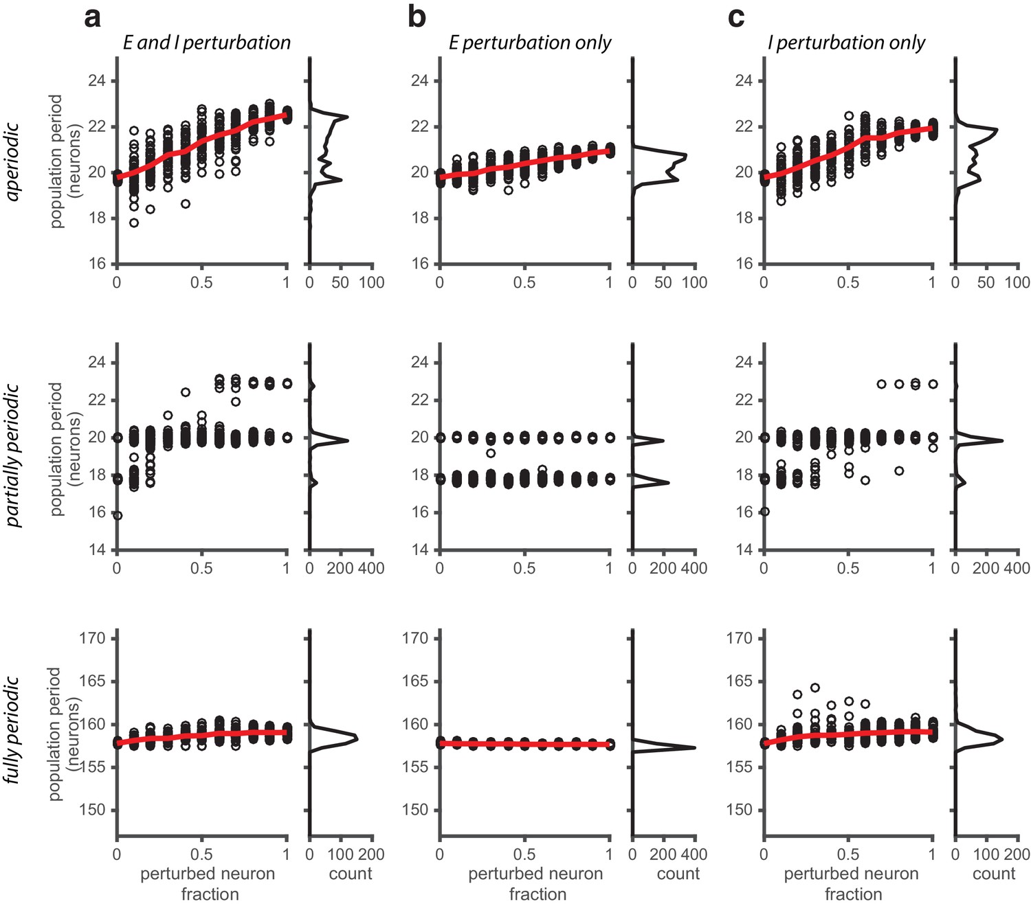
Perturbations applied to a random subset of neurons in the network.
(a) Population period as a function of a fractional perturbation of the network for aperiodic (top row), partially periodic (middle row), and fully periodic (bottom row) networks. Black circles indicate individual trials (n = 50, for each perturbation value) in which some fixed fraction of the network is randomly selected for perturbation (unperturbed neurons: ; perturbed neurons: ). For each trial, the network is driven with inputs simulating animal motion at constant speed (v = 0.3 m/s) for 10 s (see Materials and methods for definition of population period). Red line is the mean. Right: Histogram of population periods shown at left. (b–c) Same as in (a), except that the perturbation is applied to the E population (b) and I population (c) separately.
Figure 5—figure supplement 2

Perturbations applied separately to the excitatory and inhibitory populations.
(a) Left: Population period as a function of a global perturbation of the synaptic time constants (, where ms and is the perturbation parameter scale factor), for aperiodic (top row), partially periodic (middle row), and fully periodic (bottom row) networks. Black circles indicate individual trials (, for each perturbation value) in which the network is driven with inputs simulating animal motion at constant speed ( m/s) for 10 s (see Materials and methods for definition of population period). Red line is the mean. Right: Histogram of population periods shown at left. (b–c) Same as in (a), except that the perturbation is applied to the E population (b) and I population (c) separately.
Figure 5—figure supplement 3
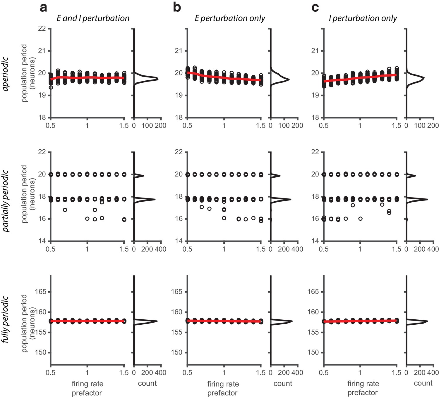
Perturbations applied to the gain of the neural response.
(a) Left: Population period as a function of a global perturbation of the firing rates (the perturbation scale factor is applied multiplicatively to both and , see Materials and methods), for aperiodic (top row), partially periodic (middle row), and fully periodic (bottom row) networks. Black circles indicate individual trials (n = 50, for each perturbation value) in which the network is driven with inputs simulating animal motion at constant speed (v = 0.3 m/s) for 10 s (see Materials and methods for definition of population period). Red line is the mean. Right: Histogram of population periods shown at left. (b–c) Same as in (a), except that the firing rate perturbation is applied to the E (b) and I (c) populations separately.
Figure 5—figure supplement 4
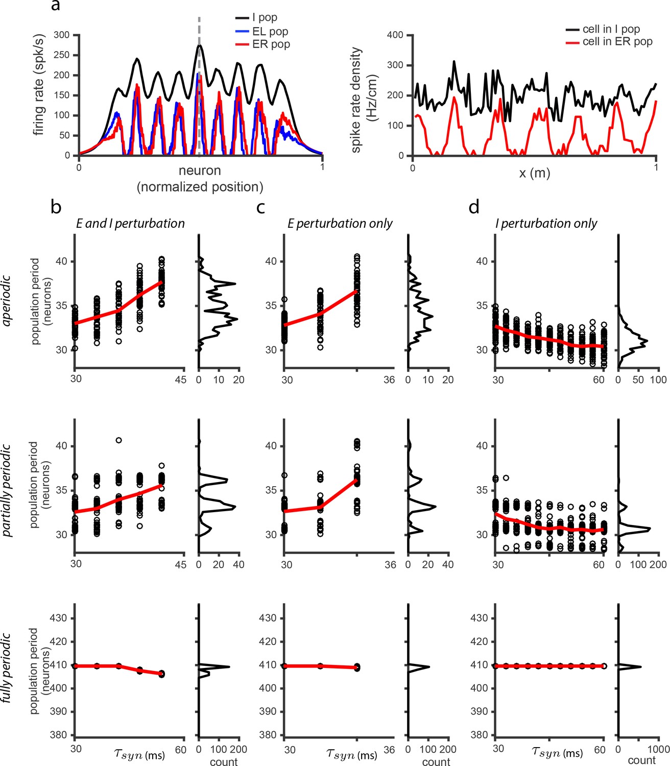
The effects of perturbations in networks with spatially untuned inhibitory neurons.
(a) Left: Snapshot of the I (black), E (red), and E (blue) population activities, for the case when EE connections are added (i.e., E-E, E-E, E-E, E-E - see Materials and methods for details; network very similar to that shown in the SI of Widloski and Fiete, 2014) and weights adjusted so that there is patterning in the E populations but not in the I population. Right: Sample single neuron spatial responses of cells in the I (black) and E (red) populations (dotted vertical line in left panel indicates relative locations of cells in the population), in the case in which the network is driven with inputs simulating a 10 s sinusoidal, back-and-forth motion of the animal across the environment. (b) Left: Population period as a function of a global perturbation of the synaptic time constants (, where ms and is the perturbation parameter scale factor), for aperiodic (top row), partially periodic (middle row), and fully periodic (bottom row) networks with additional EE connections. Black circles indicate individual trials (, for each perturbation value) in which the network is driven with inputs simulating animal motion at constant speed ( m/s) for 10 s (see Materials and methods for definition of population period). Red line is the mean. Right: Histogram of population periods shown at left. Because of the recurrent excitation in the network, perturbations can lead to very large firing rates. Therefore, we include a cap on the maximum allowable mean firing rates, which is the reason for the limited range of perturbation values in (b) and (c) for which there is data, as compared to Figure 5—figure supplement 2. (c–d) Same as in (b), except that the perturbation is applied to the E population (b) and I population (c) separately. Results: If the time-constants of all cells in this model are perturbed, the predicted effects in (b) are qualitatively the same as in Figure 5—figure supplement 2. If only E cells are affected by the perturbation, the qualitative effect in (c) is also the same as in Figure 5—figure supplement 2. If only I cells are affected, this model predicts a weak change in the opposite direction with respect to the period of the pattern relative to Figure 5—figure supplement 2: increasing perturbation in the I population leads to a decrease in the period. However, the DRPS will change in qualitatively the same way because it depends on the magnitude of change, not the sign.
Figure 5—figure supplement 5

Learned place cell-based intrinsic error correction/resetting of grid phase in familiar environments is not predicted to play an important role in novel environments according to model.
(a) Top row: Firing field of a single place cell (cell 67) learned in two familiar environments (first and second column) based on associating this field with the co-active grid cells (see Materials and methods for details; simulation based on Sreenivasan and Fiete, 2011), and the (untrained) response of this cell in a novel environment (last column). The solid vertical lines in the two familiar environments indicate the cell’s place preference. The dashed horizontal lines indicate the spiking threshold. Bottom rows: Strength of spatial inputs from grid cells of different modules (different rows) onto a single place cell (cell 67). Each colored line represents a different grid cell’s activation, multiplied by the synaptic weight from that grid cell onto place cell 67. The periodicity of the th module is (fractions of the unit-sized enclosure). In the two familiar environments, the grid cell inputs are selected by plasticity to align such that the firing field of the place cell is unimodal and above threshold at the chosen locations; in the novel environment, starting from a random arrangement of grid phases, the place cell drive does not exceed the firing threshold. Thus, it cannot reset grid cell phases to take on values from the familiar environments. (b) Sub-threshold and super-threshold (spiking) fields of entire population of place cells. Top row: Same as top row in (a), except for an entire population of place cell with learned fields, ordered according to learned location preference (in the novel environment, cells are ordered as in familiar environment 1). Bottom row: Superthreshold responses generated from the subthreshold fields in the top row by applying the spiking threshold (dashed horizontal line in (a)).
Additional files
-
Transparent reporting form
- https://doi.org/10.7554/eLife.33503.020
Download links
A two-part list of links to download the article, or parts of the article, in various formats.
Downloads (link to download the article as PDF)
Open citations (links to open the citations from this article in various online reference manager services)
Cite this article (links to download the citations from this article in formats compatible with various reference manager tools)
Inferring circuit mechanisms from sparse neural recording and global perturbation in grid cells
eLife 7:e33503.
https://doi.org/10.7554/eLife.33503


