A neural-level model of spatial memory and imagery
- University College London, United Kingdom
Figures
Figure 1

Simplified model schematic.
(A) Processed sensory inputs reach parietal areas and support an egocentric representation of the local environment (in a head-centered frame of reference). Retrosplenial cortex uses current head or gaze direction to perform the transformation from egocentric to allocentric coding. At a given location, environmental layout is represented as an allocentric code by activity in a set of BVCs, the place cells (PCs) corresponding to the location, and perirhinal neurons representing boundary identities (in a familiar environment, all these representations are associated via Hebbian learning to form an attractor network). Black arrows indicate the flow of information during perception and memory encoding (bottom-up). Dotted arrows indicate the reverse flow of information, reconstructing the parietal representation from view-point invariant memory (imagery, top-down). (B) Illustration of the egocentric (left panel) and allocentric frame of reference (right panel), where the vector s indicates South (an arbitrary reference direction) and the angle a is coded for by head direction cells, which modulate the transformation circuit. This allows BVCs and PCs to code for location within a given environmental layout irrespective of the agent’s head direction (HD). The place field (PF, black circle) of an example PC is shown together with possible BVC inputs driving the PC (broad grey arrows).
Figure 2 with 1 supplement
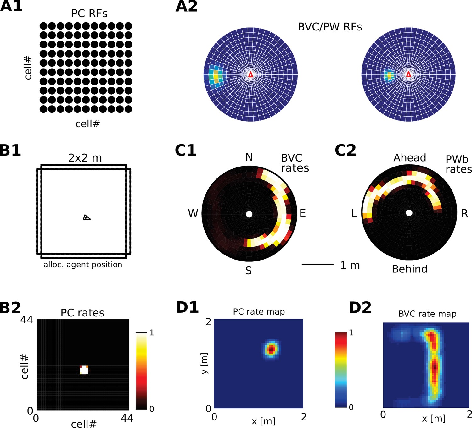
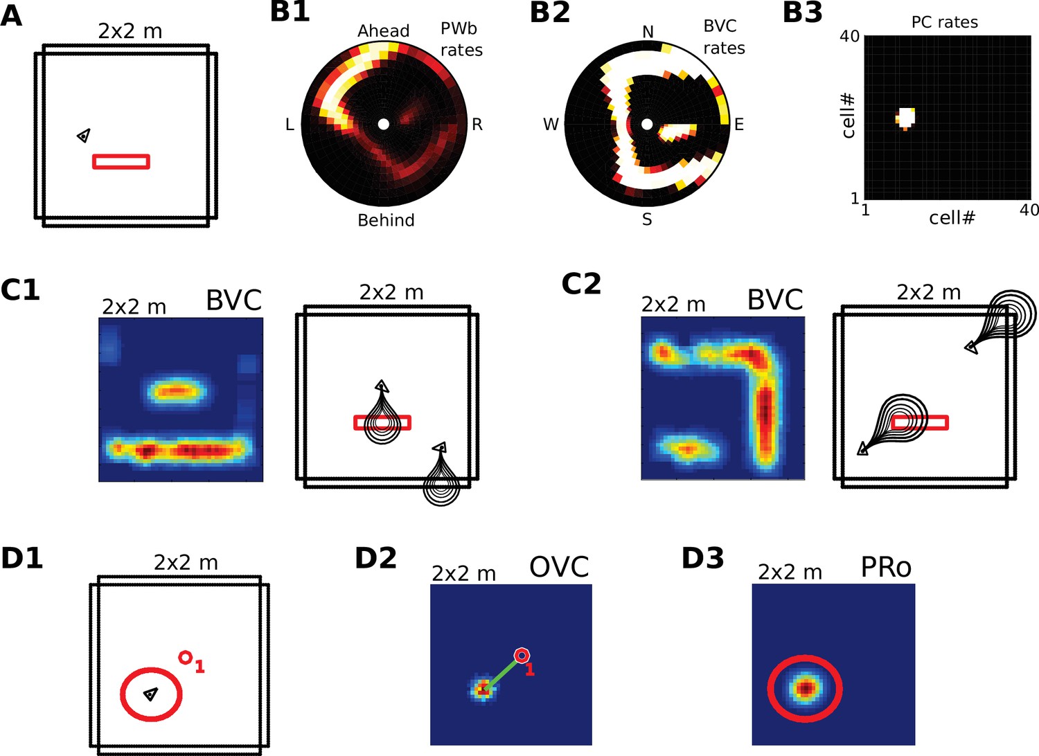
Receptive field topology and visualization of neural activity.
(A1) Illustration of the distribution of receptive field centers (RFs) of place cells (PCs), which tile the environment. (A2) Receptive fields of boundary responsive neurons, be they allocentric (BVCs) or egocentric (PWb neurons), are distributed on a polar grid, with individual receptive fields centered on each delineated polygon. Two example receptive fields (calculated according to Equation 14) are overlaid (bright colors) on the polar grids for illustration. Note that each receptive field covers multiple polygons, that is neighboring receptive fields overlap. The polar grids of receptive fields tile space around the agent (red arrow head at center of plots), that is they are anchored to the agent and move with it (for both BVCs and PWb neurons). In addition, for PWb neurons the polar grid of receptive fields also rotates with the agent (i.e. their tuning is egocentric). (B1) As the agent (black arrowhead) moves through an environment, place cells (B2) track its location. (B2) Snapshot of the population activity of all place cells arranged according to the topology of their firing fields (see A1). (C1,2) Snapshots of the population activity for BVCs and boundary selective PW neurons (PWb), respectively. Cells are again distributed according to the topology of their receptive fields (see A2), that is each cell is placed at the location occupied by the centre of its receptive field in peri-personal space (ahead is shown as up for PW neurons; North is shown as up for BVCs). See Section on the transformation circuit, Video 1, and Figure 2—figure supplement 1 for the mapping between PW and BVCs patterns via the transformation circuit. (D1,2) Unlike snapshots of population activity, firing rate maps show the activity of individual neurons averaged over a whole trial in which the agent explores the environment, here for a place cell (D1) and for a boundary vector cell with a receptive field due East (D2, tuning distance roughly 85 cm).
Figure 2—figure supplement 1
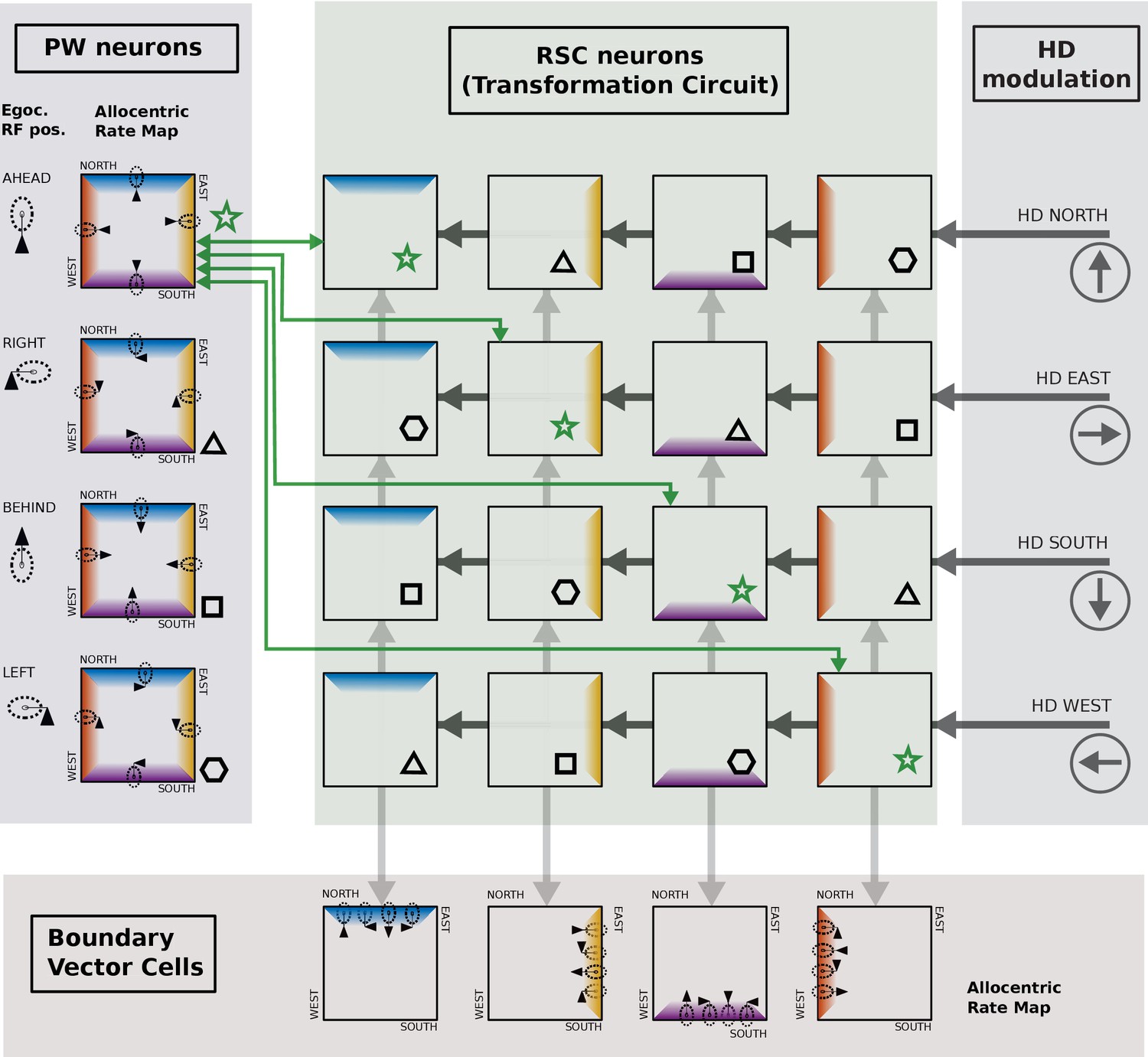
Caption: Illustration of single cell coding in the retrosplenial transformation circuit.
Shaded areas indicate the Parietal Window (PWb), the transformation circuit, head direction modulation, and boundary vector cells (BVCs). Example cells are represented as stylized firing rate maps in a simple square environment. Firing related to the North, East, South and West walls is depicted in four colors (blue, yellow, purple, red, respectively). Only 4 PWb cells, 16 transformation circuit neurons, 4 BVCs and four head-direction modulations (North, East, South, West) are shown for simplicity. PWb neurons have egocentric receptive fields (RFs, dashed ovals, shown left of and within each square) that are attached to the agent (black triangle). The RFs respond to boundaries at a specific distance and egocentric direction (ahead, left, right, behind). As the agent moves around the environment, any boundary can fall into the egocentric RF, depending on the agent’s orientation (four example positions and orientations shown), resulting in a firing rate map with firing related to all four boundaries (i.e. the blue, yellow, purple, and red bands, each conditional on the agent facing in a different direction). Considering the PWb cell with the RF ahead of the agent (top left, green star): due to the HD modulation a different RSC cell is receptive to input from that PWb neuron depending on the agent‘s current orientation. For example when the agent is facing East the 2nd row of the RSC transformation circuit is receptive to inputs from the PWb, and the first PWb neuron projects to the second cell in that row (green arrow). That RSC cell in turn projects to a BVC with a RF to the East (downward light grey arrow). The Eastward BVC also gets inputs from the other 3 PWb cells when the agent faces in the other three directions, via the other RSC neurons in the second column (connectivity not shown, but indicated by matching symbols: hexagon, triangle, square). Thus, this BVC can fire whenever the agent is near to the East wall, irrespective of the agent’s orientation. In top-down mode (imagery), PWb cells are driven by different BVCs depending on the facing direction of the animal. The PWb cell with the RF ahead of the agent (top left, green star) recieves connections from all transformation circuit neurons shown with star symbols: conveying input from the Eastward BVC when facing East, the Northward BVC when facing North etc. In this way, it is driven to fire whenever there is a boundary ahead of the agent. All connections between PWb and BVC cells and transformation circuit neurons are bidirectional, to enable both bottom-up and top-down operation.
Figure 3
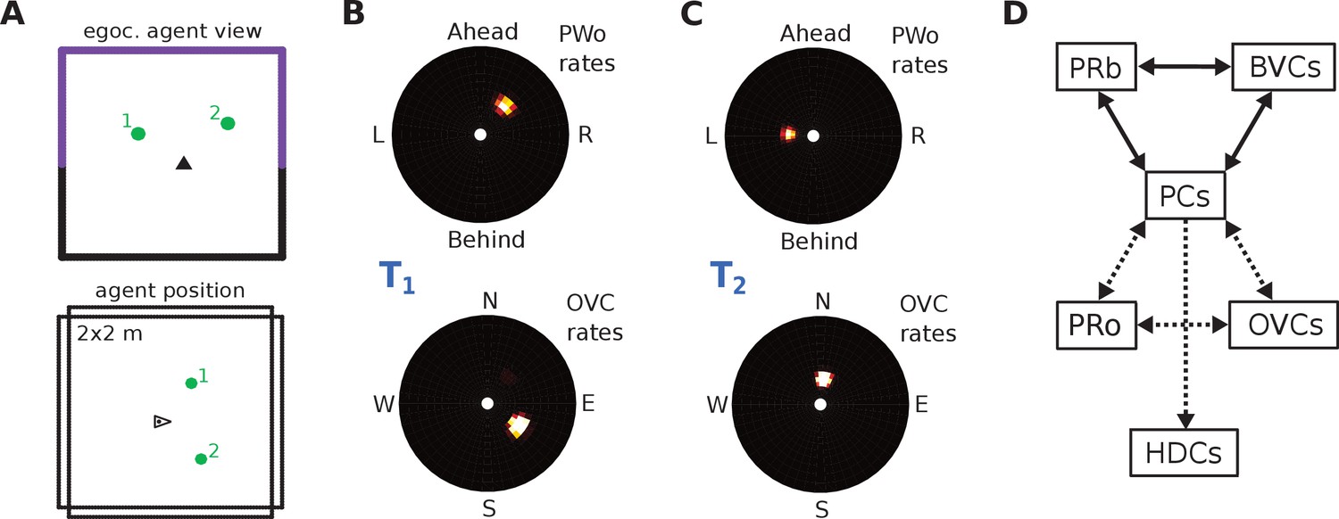
The agent model and population snapshots for object representations.
(A) Top panel: The egocentric field of view of the agent (black arrow head). Purple boundaries fall into the forward-facing 180 degree field of view and provide bottom-up drive to the parietal window (PWb; not shown, but see Figure 2C2). The environment contains two discrete objects (green circles). Bottom panel: Allocentric positions of the agent (black triangle) and objects (green circles). (B) Object-related parietal window (PWo) activity (top panel) and OVC activity (bottom panel) due to object 2, South-East of the agent, at time T1. (C) PWo activity (top panel) and OVC activity (bottom panel) due to object 1, North-East of the agent, at time T2. A heuristically implemented attention model ensures that only one object at a time drives the parietal window (PWo). (D) Illustration of the encoding of an object encountered in a familiar environment. Dashed connections are learned (as Hebbian weight updates) between active cells. Solid lines indicate connections learned in the training phase, representing the spatial context. Note that place cells (PCs) anchor the object representation to the spatial context.
Figure 4
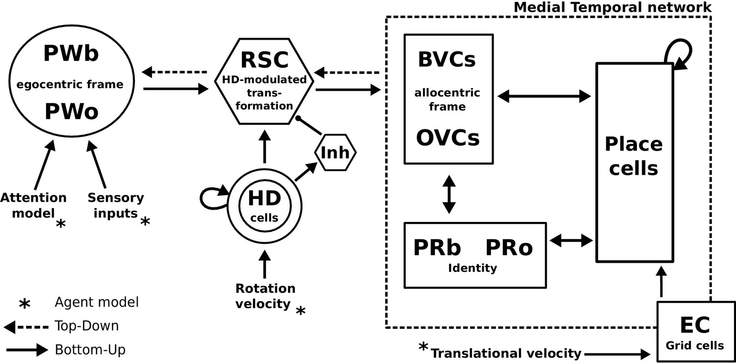
The BB-model.
‘Bottom-up’ mode of operation: Egocentric representations of extended boundaries (PWb) and discrete objects (PWo) are instantiated in the parietal window (PWb/o) based on inputs from the agent model while it explores a simple 2D environment. Attention sequentially modulates object-related PW activity to allow for unambiguous neural representations of an object at a given location. The angular velocity of the agent drives the translation of an activity packet in the head direction ring attractor network. Retrosplenial cortex (RSC) carries out the transformation from egocentric representations in the PW to allocentric representations in the MTL (driving BVCs and OVCs). The transformation circuit consists of 20 sublayers, each maximally modulated by a specific head direction while the remaining circuit is inhibited (Inh). In the medial temporal lobe network, perirhinal neurons (PRb/o) code for the identity of an object or extended boundary. PCs, BVCs and perirhinal neurons are reciprocally connected in an attractor network. Following encoding after object encounters, PCs are also reciprocally connected to OVCs and PRo neurons. ‘Top-down’ mode of operation: Activity in a subset of PCs, BVCs, and/or perirhinal neurons spreads to the rest of the MTL network (pattern completion) by virtue of intrinsic connectivity. With perceptual inputs to the PW disengaged (i.e. during recollection), the transformation circuit reconstructs parietal window (PWb/o) activity based on the current BVC and OVC activity. Updating PCs via entorhinal cortex (EC) GC inputs allows for a shift of viewpoint in imagery.
Figure 5
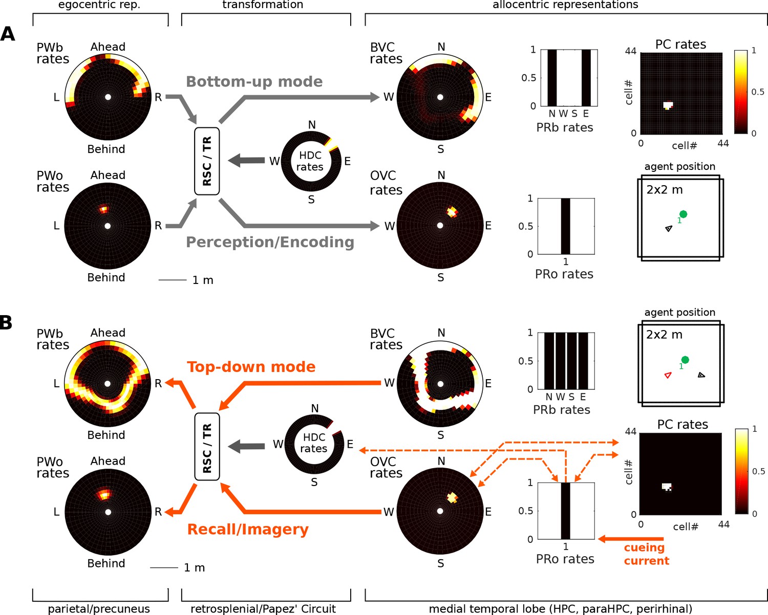
(A) Bottom-up mode of operation. Population snapshots at the moment of encoding during an encounter with a single object in a familiar spatial context. Left to right: PWb/o populations driven by sensory input project to the head-direction-modulated retrosplenial transformation circuit (RSC/TR, omitted for clarity, see Video 1 and Figure 2—figure supplement 1); The transformation circuit projects its output to BVCs and OVCs; BVCs and PRb neurons constitute the main drive to PCs; perirhinal (PRb/o) neurons are driven externally, representing object recognition in the ventral visual stream. At the moment of encoding, reciprocal connections between PCs and OVCs, OVCs and PRo neurons, PCs and PRo neurons, and PRo neurons and current head direction are learned (see Figure 3D). Right-most panels show the agent in the environment and the PC population snapshot representing current allocentric agent position. (B) Top-down mode of operation, after the agent has moved away from the object (black triangle, right-most panel). Current is injected into a PRo neuron (bottom right of panel), modelling a cue to remember the encounter with that object. This drives PCs associated to the PRo neuron at encoding (dashed orange connections show all associations learned at encoding). The connection weights switch globally from bottom-up to top-down (connections previously at 5% of their maximum value now at 100% and vice versa; orange arrows). PCs become the main drive to OVCs, BVCs and PRb neurons. BVC and OVC representations are transformed to their parietal window counterparts, thus reconstructing parietal representations (PWb/PWo) similar to those at the time of encoding (compare left-most panels in A and B). That is, the agent has reconstructed a point of view embodied by parietal window activity corresponding to the location of encoding (red triangle, right-most panel). Heat maps show population firing rates frozen in time (black: zero firing; white: maximal firing).
Figure 6
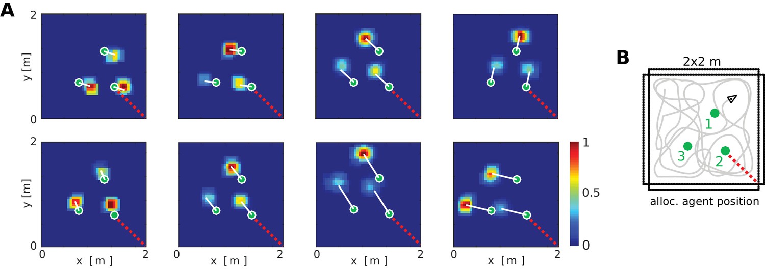
Firing fields of object vector cells.
(A) Firing rate maps for representative object vector cells (OVCs), firing for objects with a fixed allocentric location and direction relative to the agent. Object locations superimposed as green circles. Note that the objects have different identities, which would be captured by perirhinal neurons, not OVCs. Compare to Figure 4 in Deshmukh and Knierim, 2013. White lines point from objects to firing fields. Red dotted line added for comparison with B. (B) Distribution of the objects in the arena and an illustration of a possible agent trajectory.
Figure 7
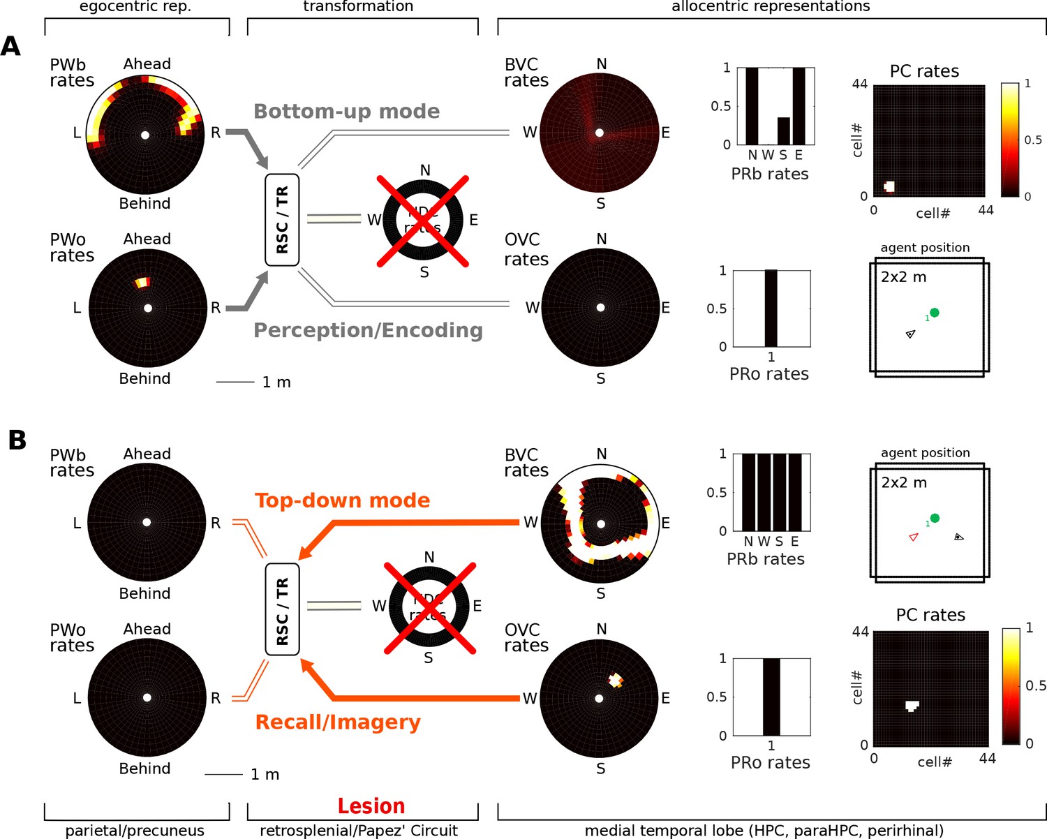
Papez’ circuit lesions.
(A) In the bottom-up mode of operation (perception), a lesion to the head direction circuit removes drive to the transformation circuit and consequently to the boundary vector cells (BVCs) and object vector cells (OVCs). A perceived object (present in the egocentric parietal representation, PWo) cannot elicit activity in the MTL and thus cannot be encoded into long-term memory, causing anterograde amnesia. Place cells fire at random locations, driven by perirhinal neurons. (B) For memories of an object encountered before the lesion, place cells can be cued by perirhinal neurons, and pattern completion recruits associated OVC, BVCs and perirhinal neurons, but no meaningful representation can be instantiated in parietal areas, preventing episodic recollection/imagery (retrograde amnesia for hippocampus-dependent memories).
Figure 8
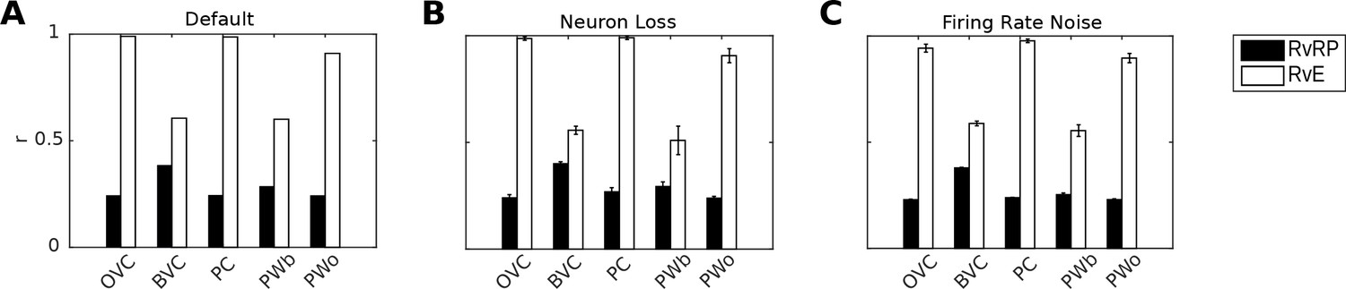
Correlation of neural population vectors between recall/imagery and encoding.
(A) In the intact model, OVCs and place cells exhibit correlation values close to one, indicating faithful reproduction of patterns. (B) Random neuron loss (20% of cells in all populations except for the head direction ring). (C) The effect of firing rate noise. Noise is also applied to all 20 retrosplenial transformation circuit sublayers (as is neuron loss; correlations not shown for clarity). Firing rate noise is implemented as excursions from the momentary firing rate as determined by the regular inputs to a given cell (up to peak firing rate). The amplitudes of perturbations are normally distributed (mean 20%, standard deviation 5%) and applied multiplicatively at each time step). White bars show the correlation between the neural patterns at encoding vs recall (RvE), while black bars show the average correlation between the neural patterns at recall vs pattern sampled at random times/locations (here every 100 ms; RvRP). Each bar is averaged over 20 separate instances of the same simulation (with newly drawn random numbers). Error bars indicate standard deviation across simulations.
Figure 9

Detection of moved objects via OVC firing mismatch.
(A) Two objects are encoded from a given location (left). After encoding, object one is moved further North. When the agent returns to the encoding location, the perceived position of object one differs from that at encoding (blue line, middle panel). When the agent initiates recall (right) the perceived location of object 1 (green filled circle) and its imagined location (end point of blue line) differ. (B) PC activity is the same in all three circumstances, that is PC activity alone is insufficient to tell which object has moved. (C-D) The perceived location as represented by OVCs during perception (C; objects 1 and 2 sampled sequentially at times T1, T2) and during recall (D; objects 1 and 2 sampled sequentially at times T3, T4). Blue circle in panel D indicates the previously perceived position of object 1. Inset bar graphs show the concurrent activity of perirhinal cells (PRo). (E) The mismatch in OVC firing results in near zero correlation between encoding and recall patterns for object 1 (black bar), while object 2 (white bar) exhibits a strong correlation, so that object one would be preferentially explored. Note, the correlation for object two is less than 1 because of the residual OVC activity of the other object (secondary peaks in both panels in D, driven by learned PC-to-OVC connections). (F) A hippocampal lesion removes PC population activity, so that OVC activity is not anchored to the agent’s location at encoding. (G-H) An incidental match between learned and recalled OVC patterns can occur for either object at specific locations (red arrow heads in second panel in G), but otherwise mismatch is signaled for both objects equally and neither object receives preferential exploration.
Figure 10
‘Top-down’ activity and ‘trace’ responses.
(A) An environment containing a small barrier (red outline) has been encoded in the connection weights in the MTL, but the barrier has been removed before the agent explores the environment again. (B) Activity snapshots for PWb (B1), BVC (B2) and PC (B3) populations during exploration. The now absent barrier is weakly represented in parietal window activity due to the periodic modulation of top-down connectivity during perception, although ‘bottom-up’ sensory input due to visible boundaries still dominates (see main text). (C1) High gain for top-down connections yields BVC firing rate maps with trace fields due to the missing boundary. Left: BVC firing rate map. Right: An illustration of the BVC receptive field (teardrop shape attached to the agent at a fixed allocentric direction and distance) with the agent shown at two locations where the cell in the left panel fires maximally. (C2) Same as C1 for a cell whose receptive field is tuned to a different allocentric direction. (D1) Similarly to the missing boundary in A, a missing object (small red circle) can produce ‘trace’ firing in an OVC (D2). Every time the agent traverses the location from which the object was encoded (large red circle in D1), learned PC-to-OVC connections periodically reactivate the associated OVC. (D3) The same PCs also re-activate the associated perirhinal identity cell (PRo), yielding a spatial trace firing field for a nominally non-spatial perirhinal cell (red circle).
Figure 11

Inspecting scene elements in imagery.
The agent encounters two objects. (A) Activity in PWo (left) and OVCs (right) populations when the agent is attending to one of the two objects during encoding. Both objects are encoded sequentially from the same location (time index 0.22 in Video 11). The agent then moves past the objects. (B) Imagery is engaged by querying for object 1, raising activity in corresponding PRo neurons (far right) and switching into top-down mode (similar to Simulation 1.0, Figure 5 and Video 2), leading to full imagery from the point of view at encoding. Residual activity in the OVC population at the location of object 2 (encoded from the same position, that is driven by the same place cells) translates to weak residual activity in the PWo population. (C) Applying additional current (i.e. allocating attention) to the PWo cells showing residual activity at the location of object 2 (leftmost blue arrow) and removing the drive to the PRo neuron corresponding to object 1 (because the initial query has been resolved) leads to a build-up of activity at the location of object two in the OVC population (blue arrow between PWo and OVC plots). By virtue of the OVC to PRo connections (blue between OVC and Pro plots), the PRo neuron for object two is driven (and inhibits PRo neuron 1, right-most blue arrows). Thus, the agent has inferred the identity of object 2, after having initiated imagery to visualize object 1, by paying attention to its egocentric location in imagery.
Figure 12
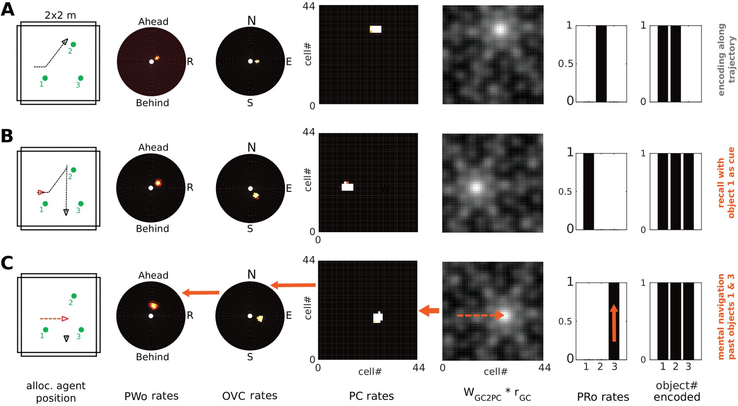
Mental navigation with grid cells.
Left to right: allocentric agent position (black triangle) and recent trajectory (black dashed line); PWo, OVC, and PC population snapshots; GC input to PCs (i.e. GC firing rates multiplied by connection weights from GCs to PCs); PRo neurons. The rightmost panel indicates which objects have been encoded. (A) The agent is exploring the environment and has just encoded the second object into memory (right-most bar chart). Object one has been encoded near the start of the trajectory. (B) After encoding the third object and moving past it, the agent initiates imagery, recalling object one in its spatial context (top-down mode) from a point of view West of object 1, facing East (red triangle). (C) Mock motor efference shifts GC activity (dashed arrow on GC input to PCs) and thence drives the PC activity bump representing (imagined) agent location. The allocentric (BVCs) and egocentric (PWb) boundary representation follow suit (see main text and Video 12). As the PC activity bump passes the location at which object 3 was encoded, corresponding OVC activity is elicited by learned connections (and is transformed into PWo activity (solid orange arrows indicate GCs updating PCs, PCs updating OVCs, etc). NB object 3 appears in the reconstructed scene ahead-right of the agent (PWo snapshot, second panel), despite being encoded ahead-left of the agent when it moved southwards from object 2 toward object 3. The corresponding perirhinal neuron is also driven to fire by PCs (orange arrow in PRo panel).
Figure 13
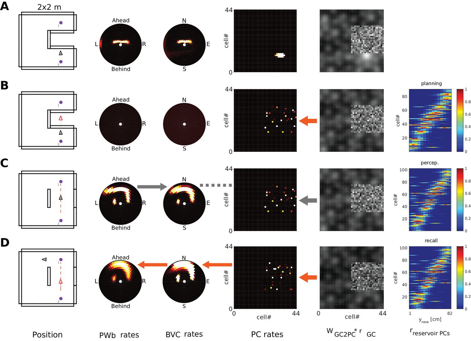
Planning, taking and imaging a trajectory across an unexplored area.
The agent is located in an environment where the direct trajectory between two salient locations (purple dots, left column) covers an unexplored part of the environment. PCs potentially firing in the unexplored area (‘reservoir cells’) receive only random connections from GCs (see unstructured grid cell input in column 5). Left to right panel columns: allocentric agent position (triangle); PWb, BVC, PC population rates; GC inputs to PCs (see Figure 12); and (B-D only) firing of ‘reservoir’ PCs along the trajectory (x axis), stacked and ordered by time of peak firing along the trajectory (y axis). (A) Starting situation. (B) Phase 1; imagined movement across the obstructed space leads to preplay-like activity in reservoir PCs (rightmost panel). Red arrow indicates the reservoir PCs are driven by grid cells. No egocentric representation can be generated from BVCs because ‘reservoir’ PCs have no connections to BVCs, that is they are not yet part of the MTL attractor. (C) Phase 2; the barrier is removed and the agent navigates the trajectory in real space. GCs again drive PCs (thick grey arrow), so the temporal sequence of reservoir cell activity in (A) is recapitulated in the spatial sequence of PC activity. Sensory inputs drive the PW (bottom-up mode) and hence BVCs (grey arrow between panels 2 and 3). Hebbian learning proceeds between PCs and BVCs (dashed grey line), and from GCs to PCs (reinforcing the drive from GCs to PCs, grey arrow between panels 4 and 5). (D) Phase 3; having traversed the novel part of the environment, the agent initiates imagery and performs mental navigation along the newly learned trajectory. The learned connections now instantiate the correct BVC and PW activity in top-down mode (orange arrows indicating flow of information, similar to Figure 12).
Author response image 1
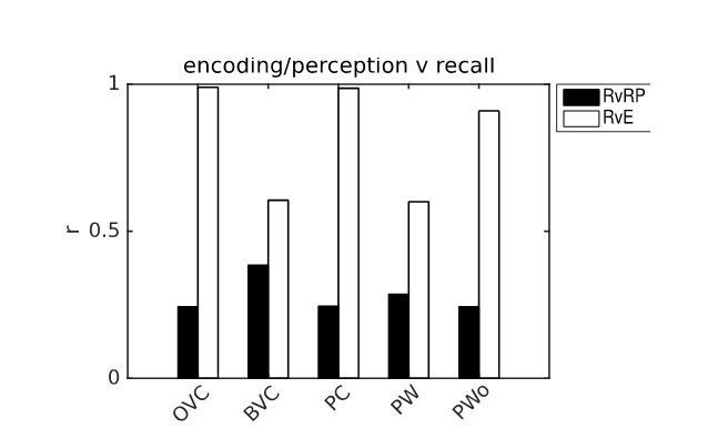
Example of pattern comparison via correlations of population vectors from simulation 1.0 (object cued recall).
White bars show the correlation between the neural patterns during imagery/recall and those during encoding (RvE), while black bars show the average correlation between the neural patterns during imagery/recall and random patterns (sampled every 100 ms; RvRP). Note that OVCs and PCs exhibit correlation values close to one, indicating faithful reproduction of patterns. BVC correlations are somewhat diminished because recall fully reactivates all boundaries indiscriminately compared to a limited field of view during perception with only modest reactivation outside the field of view. PW neurons show correlations below one because at recall reinstatement in parietal areas requires the egocentric allocentric transformation (i.e. OVC signals passed through retrosplenial cells), which smears out the pattern compared to perceptual instatement in the parietal window (i.e. imagined representations are not as precise as their counterparts during perception).
Videos
Video 1
Surface plots (heat maps) visualize theneural activity of populations of cells.
The video shows a visualization of the simulated neural activity in the retrosplenial transformation circuit as a simulated agent moves in a simple, familiar environment (See Figure 2-figure supplement 1 for further details). Individual sublayers of the transformation circuit are shown in a circular arrangement around the head direction ring. Head direction cells track the agent's heading and confer a gain modulation on the retrosplenial sublayers. The transformation circuit then drives boundary vector cells (see main text). Surface plots (heat maps) visualize the neural activity of populations of cells. Individual cells correspond to pixels/polygons on the heat maps (compare to figures). Cells are arranged according to the distribution of their receptive fields; however, this arrangement does not necessarily reflect anatomical relations. Bright colors indicate strong firing. Abbreviations: PWb, Parietal Window, egocentric boundary representations (ahead is up); HDCs, Head Direction Cells; TR, Retrosplenial transformation sublayers; BVCs, Boundary Vector Cells (North is up); egoc. agent view, egocentric field of view of the agentwithin the environment, purple outlines denote visibleboundary segments which correspond to sensoryinputs to the PWb (ahead is up); alloc. agent position, allocentric position of the agent in the environment (North is up).
Video 2
This video shows a visualization of the simulated neural activity as the agent moves in a familiar environment and encounters a novel object.
The agent approaches the object and encodes it into long-term memory. Upon navigating past the object the agent initiates recall, reinstating patterns of neural activity similar to the patterns present during the original object encounter. Recall is identified with the re-construction of the original scene in visuo-spatial imagery (see main text). Please see caption of Video 1 for abbreviations.
Video 3
This video shows the same scenario as Video 2 (object-cued recall), however, with 20% randomly chosen lesioned cells per area.
The agent moves in a familiar environment and encounters a novel object. The agent approaches the object and encodes it into long-term memory. Upon navigating past the object, the agent initiates recall, reinstating patterns of neural activity similar to the patterns present during the original object encounter. Please see caption of Video 1 for abbreviations.
Video 4
This video shows the same scenario as Video 2 (object-cued recall), however, with firing rate noise applied to all neurons (max. 20% of peak rate).
The agent moves in a familiar environment and encounters a novel object. The agent approaches the object and encodes it into long-term memory. Upon navigating past the object the agent initiates recall, reinstating patterns of neural activity similar to the patterns present during the original object encounter. Please see caption of Video 1 for abbreviations.
Video 5
This video shows a visualization of the simulated neural activity as the agent encounters an object and subsequently tries to engage recall similar to Simulation 1.0 (Video 2).
However, a lesion to the head direction system (head direction cells are found along Papez' circuit) precludes the agent from laying down new memories, because the transformation circuit cannot drive the medial temporal lobe. That is the transformation circuit cannot instantiate OVC/BVC representations derived from sensory input for subsequent encoding, leading to anterograde amnesia in the model agent (see main text). Please see caption of Video 1 for abbreviations.
Video 6
This video shows a visualization of the simulated neural activity as the agent moves through an empty environment and tries to engage recall of a previously present object.
A lesion to the head direction system (head direction cells are found along Papez' circuit) has been implemented similar to Simulation 1.1 (Video 5). The agent is supplied with the connection weights learned in Simulation 1.0 (Video 2), where it has successfully memorized a scene with an object. That is, the agent has acquired a memory before the lesion. However, even though cueing with the object re-activates the correct medial temporal representations, due to the lesion no reinstatement in the parietal window cannot occur, leading to retrograde amnesia for hippocampus-dependent memories in the model agent. Note, it is hypothesized that a cognitive agent only has conscious access to the egocentric parietal representation, as suggested by hemispatial representational negelct (Bisiach and Luzzatti, 1978) (see main text). Please see caption of Video 1 for abbreviations.
Video 7
This video shows a visualization of the simulated neural activity in a reproduction of the object novelty paradigm of Mumby et al., 2002; detecting that one of two objects has been moved).
The agent is faced with two objects and encodes them (sequentially) into memory. Following some behavior one of the two objects is moved. Note, in real experiments the animal is removed for this manipulation. In simulation, this is unnecessary. Once the agent has returned to location of encoding, it is faced with the manipulated object array. The agent then initiates recall for objects one and two in sequence. The patterns of OVC re-activation can be compared to the corresponding patterns during perception (population vectors correlated, see main text). For the moved object, the comparison signals a change (near zero correlation). That object would hence be preferentially explored by the agent, and the next movement target for the agent is set accordingly (see main text). Please see caption of Video 1 for abbreviations.
Video 8
should be compared to Video 7.
It shows a reproduction of the object novelty paradigm of Mumby et al., 2002; detecting that one of two objects has been moved). The agent is faced with two objects and encodes an association between relative object location (signaled by OVCs) and object identity (signaled by perirhinal neurons) - see Video 7 for encoding phase. Due to the hippocampal lesion, these associations cannot be bound to place cells. Once one of the two objects is moved (compare to Simulation 1.3) the agent initiates recall and the patterns of OVC re-activation are compared to the corresponding patterns during perception (population vectors correlated, see main text). Recall is initiated at two distinct locations to highlight the following effect of the lesion: Since associations between OVCs and perirhinal neurons are not bound to a specific environmental location a comparison of OVC patterns between perception and recall signals mismatch everywhere for both objects except for the two special locations at which imagery is engaged in the video. At each of those locations, the neural pattern due to the learned association happens to coincide with the pattern during perception for one of the two objects. Hence no object can be singled out for enhanced exploration. Match and Mismatch is signaled equally for both objects (see main text). Please see caption of Video 1 for abbreviations.
Video 9
This video shows a visualization of the simulated neural activity as the agent moves in a familiar environment.
However, a previously present boundary has been removed. The agent is supplied with a periodic (akin to rodent theta) modulation of the top-down connection weights (please see main text). The periodic modulation of these connections allows for a probing of the memorized spatial context without engaging in full recall and reveals the memory of the environment to be incongruent with the perceived environment. BVC activity due to the memorized (now removed) boundary periodically 'bleeds' into the egocentric parietal window ¨representation, in principle allowing the agent to attend to the part of environment which has undergone change (location of removed boundary). Time integrated neural activity from this simulation yields firing rate maps which show traces of the removed boundary (see Figure 10 in the manuscript). Note, the video is cut after 1 min to reduce filesize. The full simulation covers approximately 300 s of real time. Please see caption of Video 1 for abbreviations.
Video 10
This video shows a visualization of the simulated neural activity as the agent moves in a familiar environment.
However, a previously present (and encoded) object has been removed. The agent is supplied with a periodic (akin to rodent theta) modulation of the top-down connection weights (please see main text). The periodic modulation of these connections allows for a probing of the memorized spatial context. With every passing through the encoding location OVC activity (reflecting the now removed object) and perirhinal activity is generated by place cells covering the encoding location. This re-activation yields firing rate maps which show traces of the removed object in OVCs, and induces a spatial firing field for the nominally non-spatially selective perirhinal neuron (compare to Figure 10 in the manuscript). Note, the video is cut after 1 min to reduce filesize. The full simulation covers approximately 300 s of real time. Please see caption of Video 1 for abbreviations.
Video 11
This video shows a visualization of the simulated neural activity as the agent sequentially encodes two objects into long-term memory.
Upon navigating past the objects the agent initiates recall, cueing with the first object. The OVC representations of both objects are bound to the same place cells. These place cells thus generate a secondary peak in the OVC representation corresponding to the non-cued object. This activity propagates to the parietal window. Allocating attention to this secondary peak in the egocentric parietal representation (i.e. injecting current), propagates back to OVCs, which then drive the perirhinal cells for the non-cued object. That is, the agent infers the identity of the second object which is part of the scene (see main text). Please see caption of Video 1 for abbreviations.
Video 12
This video shows a visualization of the simulated neural activity as the agent performs a complex trajectory and encodes three objects into long-term memory along the way.
Upon navigating past the third object the agent initiates recall, cueing with the first object, and subsequently performs mental navigation (imagined movement in visuo-spatial imagery) with the help of grid cells. Grid cells update the place cell representation along the trajectory. The egocentric parietal representation is updated along the imagined trajectory, that is scene elements are flowing past the point of view of the agent. Note, the imagined trajectory does not correspond to a previously taken route. Nevertheless, when the imagined trajectory takes the agent past the encoding location of object 3, it is instantiated in the OVC and PWo representations (see main text). Grid cell firing rates are shown multiplied by their connection weights to place cells. Please see caption of Video 1 for further abbreviations.
Video 13
This video shows a visualization of the simulated neural activity as the agent performs mental navigation across a blocked shortcut.
Newly recruited cells in the hippocampus exhibit activity reminiscent of preplay. Upon removal of the barrier the agent traverses the shortcut and associates the newly recruited hippocampal cells with the perceptually driven activity in the MTL. Subsequent mental navigation across the short cut yields activity in hippocampal cells reminiscent of replay (see main text). Grid cell firing rates are shown multiplied by their connection weights to place cells. Please see caption of Video 1 for further abbreviations.
Tables
Table 1
List of simulations, their content, corresponding Figures and videos
https://doi.org/10.7554/eLife.33752.009| Simulation no. | Content | Related figures | Video no. |
|---|---|---|---|
| 0 | Activity in the transformation circuit | Figure 2—figure supplement 1 | 1 |
| 1.0 | Object-cued recall | Figures 5 and 6,8A | 2 |
| 1.0n1 | Object-cued recall with neuron loss | Figure 8B | 3 |
| 1.0n2 | Object-cued recall with firing rate noise | Figure 8C | 4 |
| 1.1 | Papez’ circuit Lesion (anterograde amnesia) | Figure 7A | 5 |
| 1.2 | Papez’ circuit Lesion (retrograde amnesia) | Figure 7B | 6 |
| 1.3 | Object novelty (intact hippocampus) | Figure 9A | 7 |
| 1.4 | Object novelty (lesioned hippocampus) | Figure 9B | 8 |
| 2.1 | Boundary trace responses | Figure 10A,B,C | 9 |
| 2.2 | Object trace responses | Figure 10D | 10 |
| 3.0 | Inspection of scene elements in imagery | Figure 11 | 11 |
| 4.0 | Mental Navigation | Figure 12 | 12 |
| 5.0 | Planning and short-cutting | Figure 13 | 13 |
Appendix 1—table 1
Model Parameters.
Top to bottom: α, β sigmoid parameters; φ connection gains; Φ constants subtracted from given weight matrices (e.g. PC to PC connections) to yield global inhibition; bath parameters; range thresholds for object encoding; l learning rates for simulation 5; S sparseness of connections for reservoir PCs; σρ, σϑ spatial dispersion of the rate function for BVCs. The additive constant (σρ = (r + 8) * σ0) corresponds to half the range of BVC grid and prevents σρ from converging to zero close to the agent. Ni population sizes. Products of numbers reflect geometric and functional aspects. E.g. receptive fields of PCs tile 2 × 2 m arena with 44 × 44 cells. Polar grids are given by 16 radial distance units (see A.2) and 51 angular distance units. For the transformation circuit this number is multiplied by the number of transformation sublayers, that is 20.
| α | 5 |
|---|---|
| β | 0.1 |
| αIP | 50 |
| βIP | 0.1 |
| φPWb-TR | 50 |
| φTR-PWb | 35 |
| φTR-BVC | 30 |
| φBVC-TR | 45 |
| φHD-HD | 15 |
| φHD-IP | 10 |
| φHD-TR | 15 |
| φHDrot | 2 |
| φIP-TR | 90 |
| φPC-PC | 25 |
| φPC-BVC | 1100 |
| φPC-PRb | 6000 |
| φBVC-PC | 440 |
| φBVC-PRb | 75 |
| φPRb-PC | 25 |
| φPRb-BVC | 1 |
| φGC-PC | 3 |
| φPWo-TR | 60 |
| φTR-PWo | 30 |
| φTR-OVC | 60 |
| φOVC-TR | 30 |
| φPC-OVC | 1.7 |
| φPRo-OVC | 6 |
| φPC-PRo | 1 |
| φOVC-PC | 5 |
| φOVC-oPR | 5 |
| φPRo-PC | 100 |
| φPRo-PRo | 115 |
| φinh-PC | 0.4 |
| φinh-BVC | 0.2 |
| φinh-PRb | 9 |
| φinh-PRo | 1 |
| φinh-HD | 0.4 |
| φinh-TR | 0.075 |
| φinh-TRo | 0.1 |
| φinh-PW | 0.1 |
| φinh-OVC | 0.5 |
| φinh-PWo | 1 |
| ΦPC-PC | 0.4 |
| ΦBVC-BVC | 0.2 |
| ΦPR-PR | 9 |
| ΦHD-HD | 0.4 |
| ΦOVC-OVC | 0.5 |
| ΦPRo-PRo | 01 |
| PWbath | 0.1 |
| PWbath | 0.2 |
| TRbath | 0.088 |
| Object enc. threshold | 18 cm |
| Object enc. Threshold (3.1) | 36 cm |
| lGC-resPC | 0.65*10^−5 |
| lresPC-BVC | 0.65*10^−5 |
| lBVC-resPC | 0.65*10^−5 |
| SGC-resPC | 3% |
| SresPC-resPC | 6% |
| σρ | (r + 8) * σ0 |
| σ0 | 0.08 |
| σϑ | 0.2236 |
| NPC | 44 × 44 |
| NBVC | 16 × 51 |
| NTRb/o | 20 × 16×51 |
| NOVC | 16 × 51 |
| NPRb/o | Dependent on simulation environment |
| NPWb/o | 16 × 51 |
| NIP | 1 |
| NHD | 100 |
| NGC | 100 per module |
| Nreservoir | 437 |
Additional files
-
Transparent reporting form
- https://doi.org/10.7554/eLife.33752.030
Download links
A two-part list of links to download the article, or parts of the article, in various formats.
Downloads (link to download the article as PDF)
Open citations (links to open the citations from this article in various online reference manager services)
Cite this article (links to download the citations from this article in formats compatible with various reference manager tools)
A neural-level model of spatial memory and imagery
eLife 7:e33752.
https://doi.org/10.7554/eLife.33752


