Figures and data in Trade-off shapes diversity in eco-evolutionary dynamics | eLife

Figures

23 figures

Figures

Figure 1

Download asset Open asset

Link between genotype, phenotype and interaction space.

This schematic shows species in a community of grain-eating and nectar-feeding birds, living in an environment where nectar feeding is advantageous. (a) Six different genotypes (sequences $S_{i}$ ) on a distance tree genotype space. (b) Four distinct phenotypes, $P_{j}$ , are present in this space. Genotypes $S_{1}$ and $S_{2}$ are mapped to the same phenotype $P_{I}$ , and $S_{5}$ and $S_{6}$ are mapped to the same phenotype $P_{I V}$ . (c) Interaction space distinguishes only three interaction traits $T_{k}$ (for definition see Model section below). $P_{I}$ and $P_{I I}$ are mapped to the same interaction trait $T_{α}$ because the change of feather color does not affect ecological interactions regarding the feeding habit. The table on the right shows how the complexity of the description reduces as we map the system to interaction space.

https://doi.org/10.7554/eLife.36273.003

Figure 2

Download asset Open asset

Trade-off between replication and competitive ability.

The shape of trade-off is controlled by trade-off parameter $δ$ (Appendix 1, Trade-off). Trade-off functions with $δ = 0$ , $0.14$ , $0.29$ , $0.43$ , $0.57$ , $0.71$ , $0.86$ are plotted, each in different color, from the dark blue horizontal line for $δ = 0$ (i.e. no trade-off), to the red convex curve for $δ = 0.86$ .

https://doi.org/10.7554/eLife.36273.004

Figure 3 with 1 supplement

Download asset Open asset

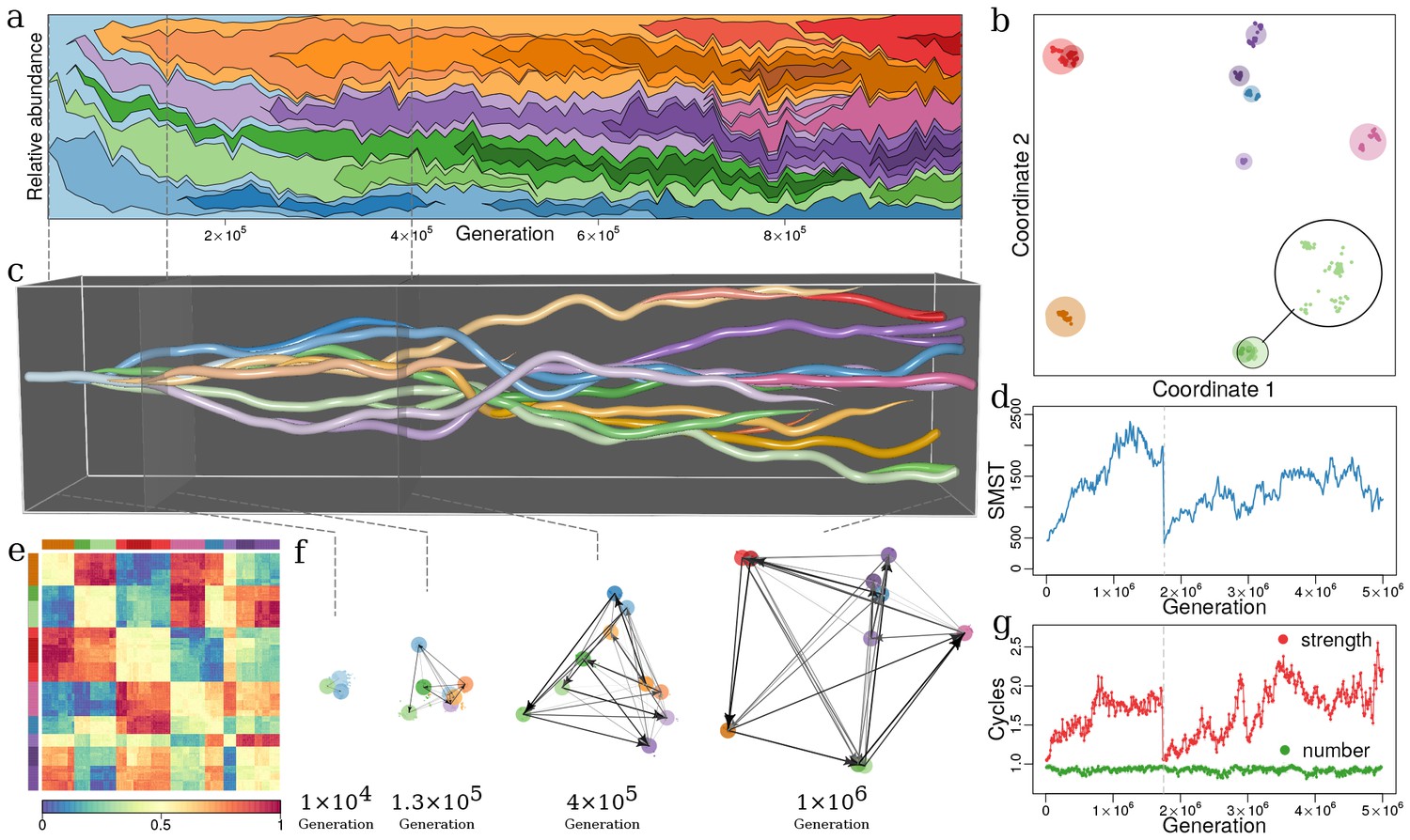
Evolutionary dynamics of a community driven by competitive interactions, with trade-off between fecundity and competitive abilities ( $δ = 0.5$ , $λ = 300$ , $μ = 0.001$ , $m = 0.02$ , $N_{s} = 10^{5}$ ).

(a) Species’ frequencies over time (Muller plot): one color per species, vertical width of each colored region is the relative abundance of respective species. Frequencies are recorded every $10^{4}$ generations over $10^{6}$ generations. The plot was produced with R-package MullerPlot (Farahpour et al., 2016). (b) Distribution over trait space: Snapshot of distribution of strains and species in trait space after $10^{6}$ generations. By using classical multidimensional scaling the multidimensional trait space is reduced to two dimensions that explain most of the variance in trait space (see Appendix 1, Classical multi-dimensional scaling (CMDS)). Points and discs are strains and species, respectively (see Appendix 1, Species and strains). Magnified disc in lower right corner shows strains in the light green species disc. Discs diameter are proportional to the total abundance of corresponding species, i.e. the sum of relative abundances of all strains that belong to that species. In this snapshot $N_{s t} = 660$ and $N_{s p} = 10$ . (c) Evolutionary dynamics in trait space: Snapshots as in panel (b), but concatenated for all times (horizontal axis), from the monomorphic first generation to generation $10^{6}$ . Figure 3—video 1 shows this evolutionary dynamics over time. (d) Functional diversity over time (see Appendix 1, Diversity indexes and parameters of dynamics) measured by the size of minimum spanning tree (SMST) in interaction trait space (see Appendix 1, SMST and distribution of species and strains in trait space). At $1.75 \times 10^{6}$ generations diversity collapses with all species but one going extinct (vertical dashed line) (Appendix 1, Collapses of diversity). (e) Heatmap of interaction matrix $I$ for generation $10^{6}$ . Row and column order reflects species consistent with panel (b) and indicated by color bars along top and left. Colors inside heat map represent values of interaction terms (color-key along bottom). (f) Evolution of dominance network: several snapshots from panel (c) with dominance edges, $W_{i j}^{s p}$ between species (colored discs). (g) Numbers and mean strength of cycles over time in green and red, respectively. The strength of a cycle is defined by its weakest edge. Number and mean strength are given in units of number and mean strength of equivalent random networks, respectively (Appendix 1, Intransitive dominance cycles). Right ends in (a) and (c) correspond to generation panel (b) and (e). Colors of species are the same in panels (a), (b), (c), (e) and (f). Note that time scales differ between panels (a), (c) and (d), (g).

https://doi.org/10.7554/eLife.36273.005

Figure 3—video 1

Download asset

posterframe for video — Divergent eco-evolutionary dynamics in interaction trait space.
https://doi.org/10.7554/eLife.36273.006

Figure 4

Download asset Open asset

Effects of trade-off $δ$ and lifespan $λ$ on community structure and diversity.

(a) Mean weight of dominance edges $⟨ W ⟩$ (orange squares) and mean strength of cycles $ρ$ (blue circles) as function of $δ$ . Mean cycle strength is given in units of mean strength of corresponding random networks for the respective trade-off (Appendix 1, Intransitive dominance cycles). Points in panel (a) are evaluated as averages over three different simulations, each over $5 \times 10^{6}$ generations with $μ = 0.001$ , $m = 0.02$ , $λ = \infty$ and $N_{S} = 10^{5}$ . Error bars are standard deviations averaged over these three simulations. The shaded area marks mean strength of cycles for a neutral model with corresponding parameters $\pm$ standard deviation. (b) Phase diagram of diversity as function of trade-off $δ$ and lifespan $λ$ . Diversity (represented by color spectrum defined in the color bar) is given as consensus of several quantities (Appendix 1, Diversity indexes and parameters of dynamics for different trade-offs and lifespans). Diversity has four distinct phases (I–IV). Insets along the top margin are representative MDS plots (Appendix 1, Classical multi-dimensional scaling (CMDS)) of strain distributions in trait space, with $λ = 10^{5}$ but different values of $δ$ (left to right: I with $δ = 0.11$ ; II with $δ = 0.5$ ; III with $δ = 0.89$ ). Panel (a) corresponds to a horizontal cross-section through the phase diagram in panel (b) with $λ = \infty$ for $⟨ W ⟩$ and $ρ$ as indicators of community structure.

https://doi.org/10.7554/eLife.36273.007

Appendix 1—figure 1

Download asset Open asset

Genealogical tree corresponding to the simulation reported in Figure 3 of the main text.

This tree contains around 80000 different strains clustered into 24 species with the threshold of $7 \times 10^{4}$ generations. Colors are the same as in Figure 3a, b, c and f of the main text. Black dots represent the strains that are present in the last snapshot of Figure 3a and b (Generation $10^{6}$ ). 10 out of 24 species are still extant in the last snapshot. Red circles show the branching points.

https://doi.org/10.7554/eLife.36273.009

Appendix 1—figure 2

Download asset Open asset

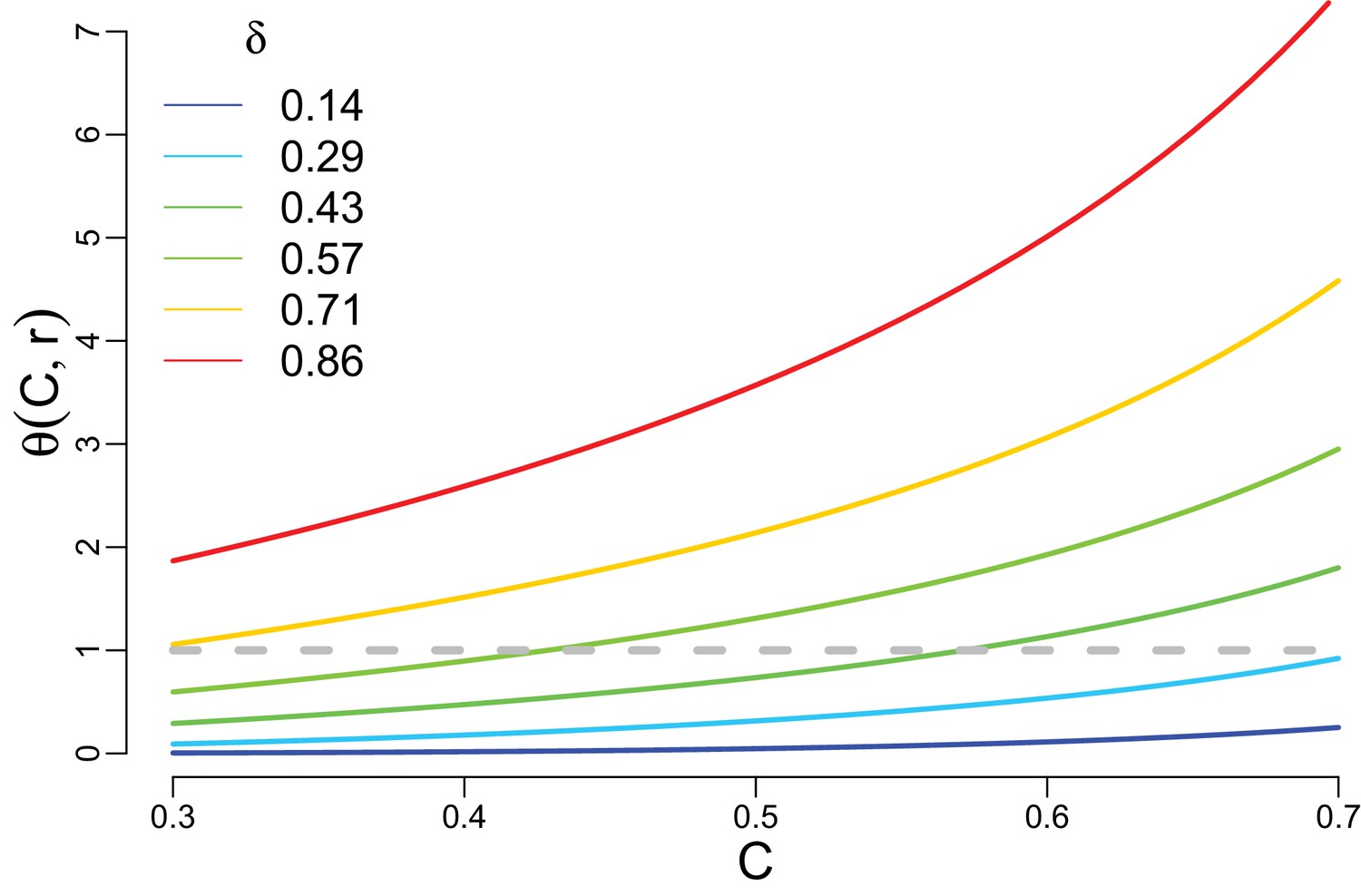
Trade-off strength $θ (C, r)$ as a function of competitive ability for different values of trade-off parameter $δ$ .

For $δ > 0.5$ , $θ (C, r)$ increases rapidly and deviates from one but for low trade-offs $θ (C, r) ≪ 1$ . Color code corresponds to the one used in Figure 2 of the main text.

https://doi.org/10.7554/eLife.36273.010

Appendix 1—figure 3

Download asset Open asset

Top-left: Trait space at generation $6 \times 10^{4}$ projected into two dimensions using CMDS.

Top-right: Percentage of variation explained by the first 20 eigenvectors from factor analysis. Here the first two eigenvectors explain around $2 \times 18 = 36$ % of variation. Bottom: Same system as the top but for generation $1 \times 10^{6}$ . Here, the first two eigenvectors explain around 78% of variation. Simulation was done with $δ = 0.5$ , $λ = 300$ , $μ = 0.001$ and $m = 0.02$ .

https://doi.org/10.7554/eLife.36273.011

Appendix 1—figure 4

Download asset Open asset

Percentage of variation explained by the first two coordinates versus time for one simulation.

Simulation was done with $δ = 0.5$ , $λ = 300$ , $μ = 0.001$ and $m = 0.02$ .

https://doi.org/10.7554/eLife.36273.012

Appendix 1—figure 5

Download asset Open asset

Minimum Spanning Tree (MST) in interaction trait space.

Left: 2D representation of MST of a typical snapshot of a simulation with $δ = 0.5$ , $λ = 300$ , $μ = 0.001$ , and $m = 0.02$ . The community in this snapshot consists of 667 strains. Here we used R-package vegan 2.4–5 to find the MST. Right: the set of 500 gray curves shows the sorted lengths of the edges of the MST versus their ranks (rank 1 = longest edge) for 500 snapshots from simulations with the aforementioned parameters. The red curve is the average of all curves and the red shaded area is the corresponding standard deviation. $R_{1}$ and $R_{2}$ are approximate lengths of short branches connecting strains within clusters ( $R_{1}$ ), and long branches ( $R_{2}$ ) connecting species. $N$ approximates the number of long branches or species.

https://doi.org/10.7554/eLife.36273.013

Appendix 1—figure 6

Download asset Open asset

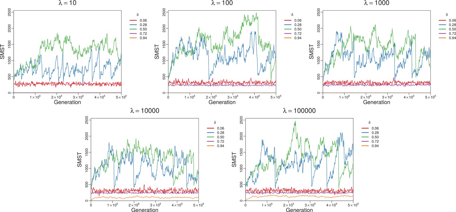
Changes of SMST over time for different trade-off parameters $δ$ but fixed lifespan $λ$ in each plot.

For very large $δ$ diverse strategies cannot be adopted. For the smallest $δ$ diverse strategies can emerge easily, but among them extreme strategies (Darwinian Demons) very quickly dominate leading to low diversity. Sustainable diversity emerges for moderate values of $δ$ . Very short lifespans $λ$ prevent increase in diversity, especially for big trade-offs (zero SMST for $λ = 10$ and high $δ$ ). Simulations were done with $μ = 0.001$ and $m = 0.02$ .

https://doi.org/10.7554/eLife.36273.014

Appendix 1—figure 7

Download asset Open asset

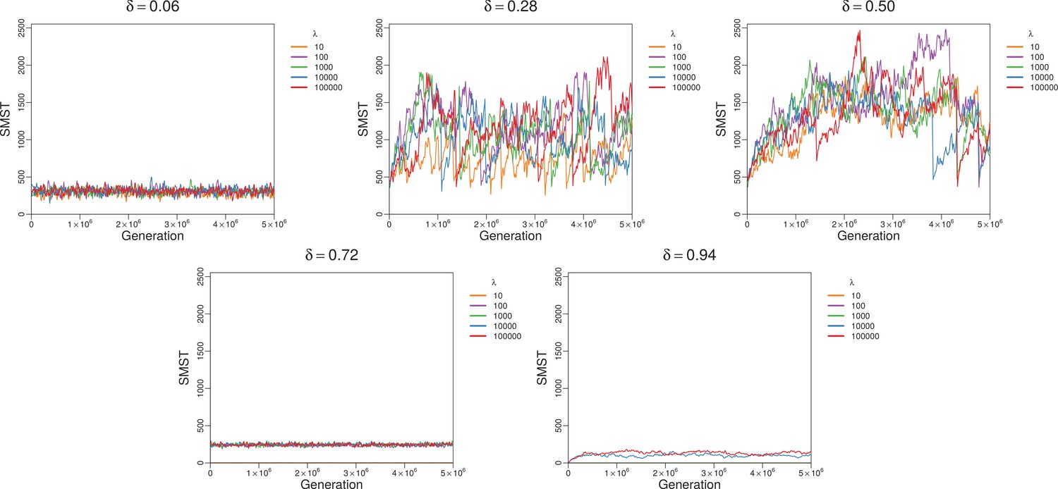
Changes of SMST over time for different lifespans $λ$ but fixed trade-off $δ$ in each plot.

Apparently lifespan has no large effect for small and moderate $δ$ . For big $δ$ , short lifespans suppress diversity completely (extinction). Simulations with $μ = 0.001$ and $m = 0.02$ .

https://doi.org/10.7554/eLife.36273.015

Appendix 1—figure 8

Download asset Open asset

Diversity indexes used to compute the phase diagram of Figure 4 of the main text.

(a) Richness: number of different strains in community. (b) Shannon entropy: here a measure of evenness in strain population. (c) Relative strength of cycles of size three compared to random networks (see Appendix 1, Intransitive dominance cycles). (d) Standard deviation of replication $r$ as a measure of diversity in reproduction strategy. (e) Functional dispersion (FDis, without using the abundance vector): measures the mean distance of individual strains in trait space to their centroid. (f) Functional dispersion (FDis, using the abundance vector): measures the mean distance of individual strains (weighted by abundance vector) in trait space to their centroid. (g) Functional evenness (FEve, using the abundance vector): quantifies functional evenness and is higher when strains/species are spread homogeneously in trait space. When disruptive selection produces clusters of localized strains in trait space this index decreases. (h) Rao’s quadratic entropy (without using the abundance vector): measures mean functional distance between two randomly chosen individuals. (i) Rao’s quadratic entropy (using the abundance vector): measures mean functional distance between two randomly chosen individuals. (j) Maximum distance in trait space between strains. (k) Volume of trait space: calculated by multiplication of eigenvalues of factor analysis. (l) SMST (see Appendix 1, SMST and distribution of species and strains in trait space). (m) Area of MDS plot: calculated by multiplication of the two first eigenvalues of factor analysis. (n) Standard deviation of interaction terms. (o) Community population: number of individuals in community. (p) Number of mass extinction events over $5 \times 10^{6}$ generations. Each plot is the average of corresponding index over three simulations each over $5 \times 10^{6}$ generations. Simulations with $μ = 0.001$ , $m = 0.02$ and $N_{s} = 10^{5}$ .

https://doi.org/10.7554/eLife.36273.016

Appendix 1—figure 9

Download asset Open asset

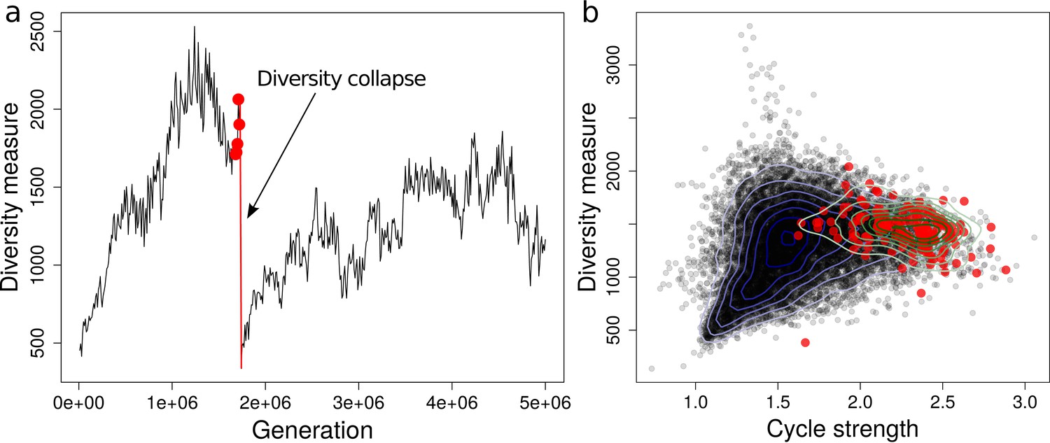
(a) Diversity collapse in a sample simulation with $δ = 0.4$ , $λ = 3 \times 10^{4}$ , $μ = 0.001$ and $m = 0.02$ .

Diversity collapse (red line) is defined as a sharp decrease in diversity. Red dots mark 5sampling time steps before the collapse. (b) Diversity versus average cycle strength for 24 different simulations each over $5 \times 10^{6}$ generations with $μ = 0.001$ , $m = 0.02$ , $δ = 0.28, 0.33, 0.4, 0.44, 0.5, 0.56$ and $λ = 1 \times 10^{4}, 3 \times 10^{4}, 1 \times 10^{5}, \infty$ . The red dots highlight the five sampling time steps before each observed collapse. The overall distribution of sampled values, and the distribution of the (red) points preceding the collapses are over plotted as two sets of contours.

https://doi.org/10.7554/eLife.36273.017

Appendix 1—figure 10

Download asset Open asset

Functional diversity, measured by size of minimum spanning tree (SMST), as function of trade-off parameter for different system sizes $N_{s}$ .

Simulations with $λ = \infty$ , $μ = 0.001$ , and $m = 0.02$ .

https://doi.org/10.7554/eLife.36273.018

Appendix 1—figure 11

Download asset Open asset

Functional diversity, measured by size of minimum spanning tree (SMST) versus size of the system in a log-log plot, averaged over middle range of trade-off parameter ( $δ = 0.44, 0.5, 0.56$ ).

We see a scaling relation with exponent of $1.97$ between diversity and size of the system. Simulations with $λ = \infty$ , $μ = 0.001$ , and $m = 0.02$ .

https://doi.org/10.7554/eLife.36273.019

Appendix 1—figure 12

Download asset Open asset

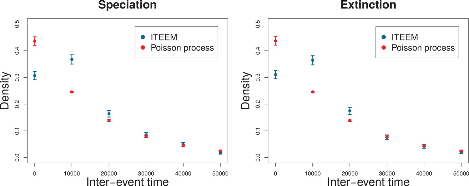
Distribution of time interval between speciation events (left) and extinction events (right).

Blue points and error bars: data from 24 ITEEM simulations, each of $5 \times 10^{6}$ generations ( $δ = 0.5, λ = 10^{5} \dots \infty, N_{S} = 10^{5}, μ = 0.001, m = 0.02$ ). Error bars are $\pm 2$ standard deviations calculated by bootstrapping. Red points and error bars: maximum likelihood fit (function fitdistr in R-package MASS, version 7.3–44) of the simulated data to a geometric distribution (discrete version of an exponential distribution), corresponding to an assumed Poisson process. Error bars are $\pm 2$ standard deviations estimated by a maximum likelihood fit.

https://doi.org/10.7554/eLife.36273.020

Appendix 1—figure 13

Download asset Open asset

SMST for different mutation probabilities ( $μ$ ) versus trade-off ( $δ$ ) and lifespan ( $λ$ ).
https://doi.org/10.7554/eLife.36273.021

Appendix 1—figure 14

Download asset Open asset

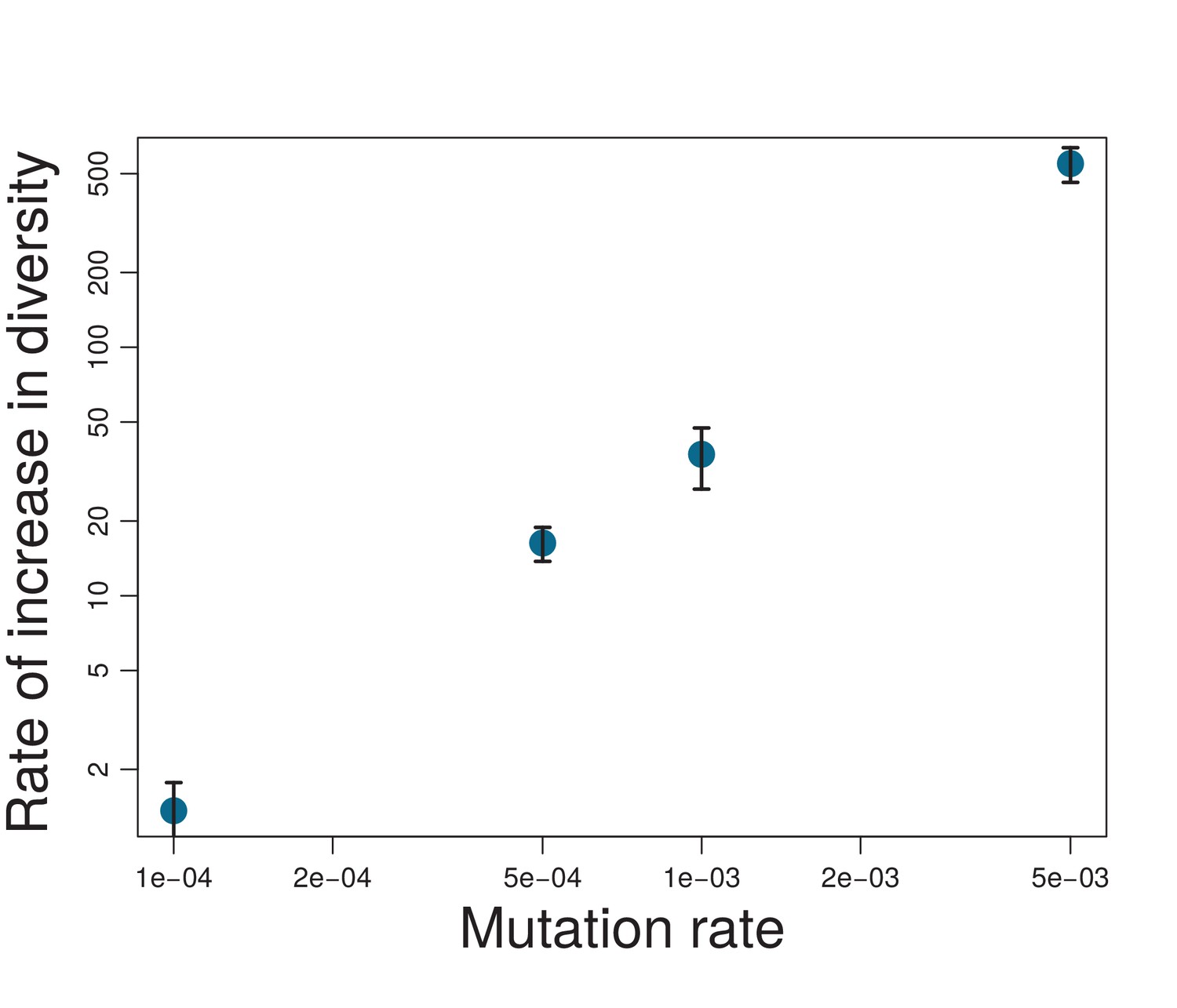
Rate of increase in diversity (measured as increase of SMST per 10000 generations) for different mutation probabilities $μ$ .

Rate of increase in diversity is calculated by fitting a line to the first 80000 generations of each simulation and averaging is over five different simulations. Error bars show the errors estimated by the fit. Note the log-log scale of the plot.

https://doi.org/10.7554/eLife.36273.022

Appendix 1—figure 15

Download asset Open asset

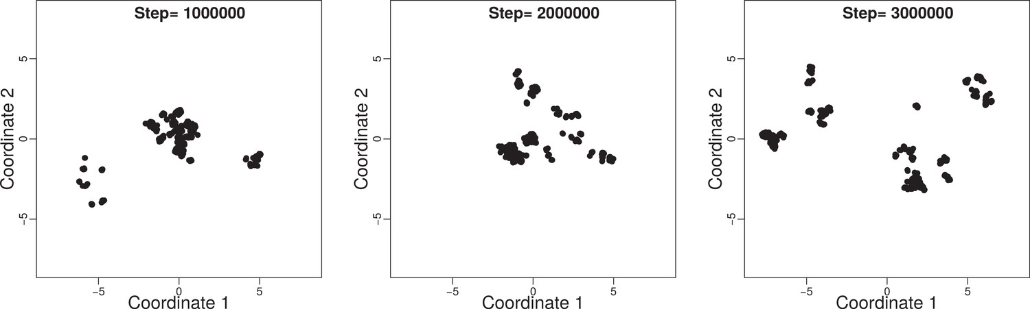
Trait space of a community evolved under neutral model at three time steps: $1 \times 10^{6}$ , $2 \times 10^{6}$ , and $3 \times 10^{6}$ with $λ = 100$ , $r = 0.9$ , $μ = 0.001$ , and $m = 0.02$ .

Note the small size of the trait space in comparison to a non-neutral model (bottom left panel of Appendix 1—figure 3).

https://doi.org/10.7554/eLife.36273.023

Appendix 1—figure 16

Download asset Open asset

Changes of SMST (top panels) and relative strength of cycles (bottom panels) over time for three different lifespans.

Colored curves are the results of the neutral model with different reproduction rates ( $r = 0.1, 0.5, 0.9$ ). The results are compared with the outcome of one simulation with $δ = 0.56$ and the corresponding lifespans (gray curves). For $λ = 10$ and $r = 0.1$ the population went extinct very quickly.

https://doi.org/10.7554/eLife.36273.024

Appendix 1—figure 17

Download asset Open asset

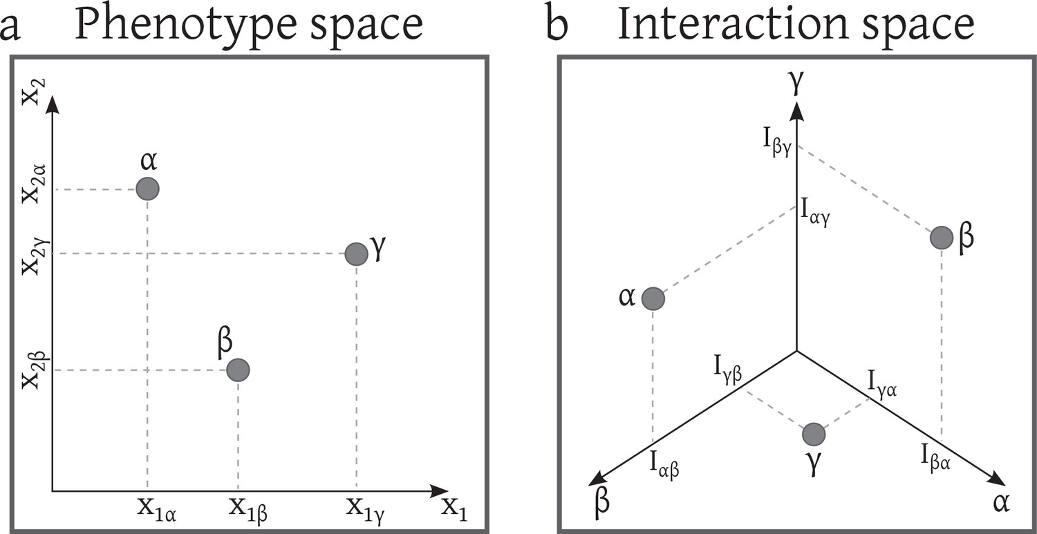
Distribution of strains in a) the phenotype space b) the interaction space.

This system consists of 3 strains with two phenotypic traits. Here, without loss of generality, we ignore intra-specific competitions. Interaction terms are obtained from the competition kernel: $I_{α β} \propto a (x_{α}, x_{β})$ .

https://doi.org/10.7554/eLife.36273.025

Appendix 1—figure 18

Download asset Open asset

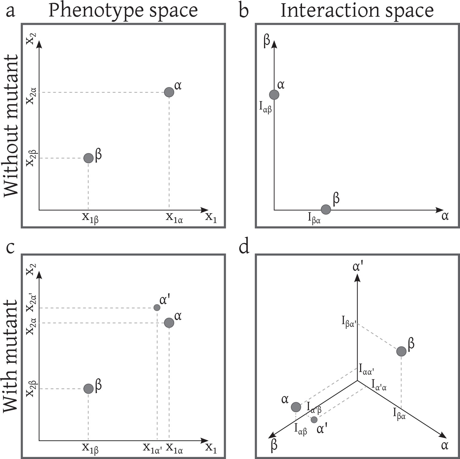
The phenotype and the interaction space of a system that first consists of 2 strains with two phenotypic traits and then is invaded by a mutant.
https://doi.org/10.7554/eLife.36273.026

Appendix 1—figure 19

Download asset Open asset

Non-injectivity of the phenotype-interaction map.

Depending on the competition kernel, several phenotype arrangements can be mapped to the same interaction arrangement. For example if we consider an asymmetric competition kernel like $a (x_{α}, x_{β}) = \sum_{i = 1, 2} d (1 - \frac{1}{1 + b e^{- c (x_{α i} - x_{β i})}})$ (Kisdi, 1999), the two imaginary phenotypes that are shown as $β$ in (a) will be mapped to the same point in the interaction space. Remember that these two are not present at the same time but both are possible phenotypic traits that give rise to the same interaction term with $α$ . In fact in this example for the aforementioned competition kernel set of points that all map to the same interaction term with $α$ form a curve (thick gray line).

https://doi.org/10.7554/eLife.36273.027

Download links

A two-part list of links to download the article, or parts of the article, in various formats.

Downloads (link to download the article as PDF)

Article PDF

Open citations (links to open the citations from this article in various online reference manager services)

Mendeley

Cite this article (links to download the citations from this article in formats compatible with various reference manager tools)

Farnoush Farahpour
Mohammadkarim Saeedghalati
Verena S Brauer
Daniel Hoffmann

(2018)

Trade-off shapes diversity in eco-evolutionary dynamics

eLife 7:e36273.

https://doi.org/10.7554/eLife.36273

Sign up for email alerts

Privacy notice