A time-stamp mechanism may provide temporal information necessary for egocentric to allocentric spatial transformations
- University of Ottawa, Canada
Figures
Figure 1 with 4 supplements
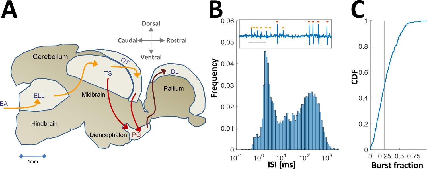
Neural recordings in PG.
(A) Electrosensory pathways from periphery to telencephalon. EA, Electrosensory afferents; ELL, electrosensory lobe; TS, Torus semicircularis (similar to the inferior colliculus); OT, optic tectum (homolog of the superior colliculus); PG, preglomerular complex; DL, dorsolateral pallium. (B) Interspike-interval (ISI) distribution in an example PG cell. Note peak around 2 ms due to thalamic-like bursting. Inset: extracellular voltage example depicting two units (red and yellow markers); scale-bar, 5 ms. (C) Cumulative distribution function of burst fraction (see Materials and methods) for all PG single-units; median = 0.24.
Figure 1—figure supplement 1
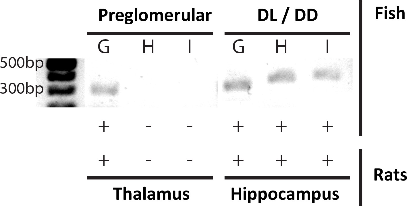
T-type Ca2+ channel expression profiles support PG thalamic homology.
mRNA expression of G, H and I subtypes of the T-type Ca2+ channel α-unit, for PG (left) and the pallial DL-DD region (right) of A. leptorhynchus – compared with mRNA expression of the same subunits in the thalamus and hippocampus of rats (Talley et al., 1999). Only the α1G transcript of the T type Ca2+ channel (CaVT) is expressed in both PG and thalamic neurons; in contrast, all three transcripts are expressed in DL and hippocampal neurons. We propose that PG spike bursting (Figure 1B,C) is generated by the α1G T-type Ca2+ channels and that this is a highly conserved biophysical/genetic feature of neurons in the vertebrate thalamus.
Figure 1—figure supplement 2

Dataset summary.
(A) Table showing, for each of the 84 single-units reported in this study, which of the electrolocation protocols were used (gray). These protocols are (from left to right): Receptive field mapping (Figure 2); Longitudinal motion (Figure 3A–B); Intermittent longitudinal motion (Figure 3C); Transverse motion (Figure 3D–F); Brass/plastic comparison (Figure 4); Random Interval (Figure 5A–C); Oddball (Figure 5D–F). Due to technical limitations, cells were tested either with longitudinal or with transverse motion protocols, but not both. (B) Table showing, for each experiment cited in this study, the number of individual penetrations, the total number of recording sites (from all penetrations), the total number of motion-responsive single-units recorded and the protocols used throughout the experiment.
Figure 1—figure supplement 3
Spike sorting example.
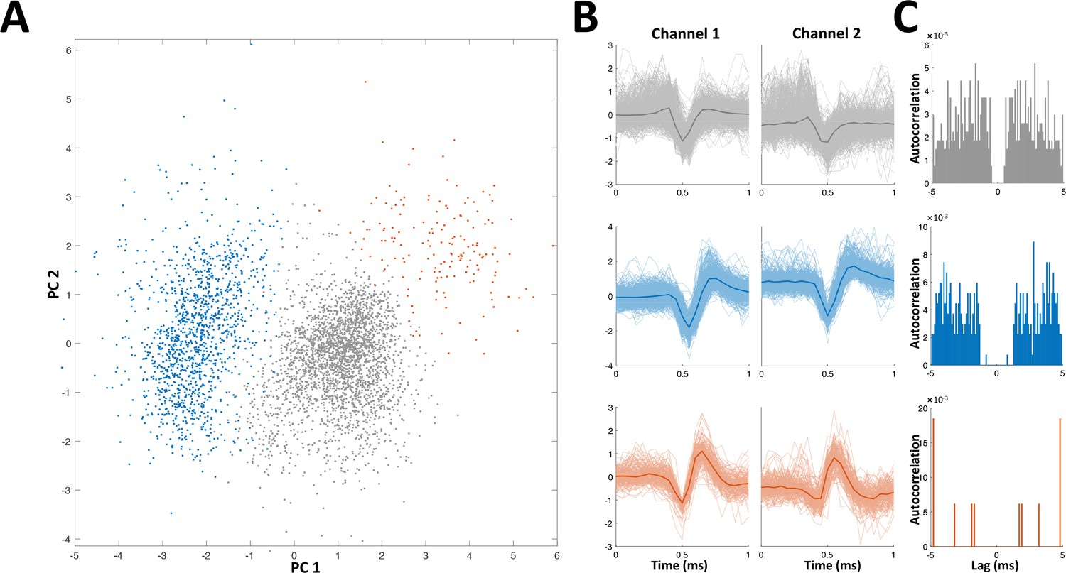
Recordings were made using either stereotrodes (two wire bundles) or tritrodes (three wire bundles); one wire was used as reference, so that near perfect cancelation of the electric organ discharge (EOD) interference was obtained. Recordings therefore consisted of either one or two channels. In the depicted example two channels (i.e., a tritrode) were employed. (A) Distribution of first two principal components of detected spikes, color coded according to unit identity (grey- multi-unit, blue and red- single units). (B) Spike shapes in the two recording channels for each unit (color codes as in panel A). (C) Autocorrelations of spiking activity in the three units. Single units (blue and red) are characterized by a refractory period (larger than the refractory period set for the spike detection algorithm, 1 ms).
Figure 1—figure supplement 4
Localization of recorded units.
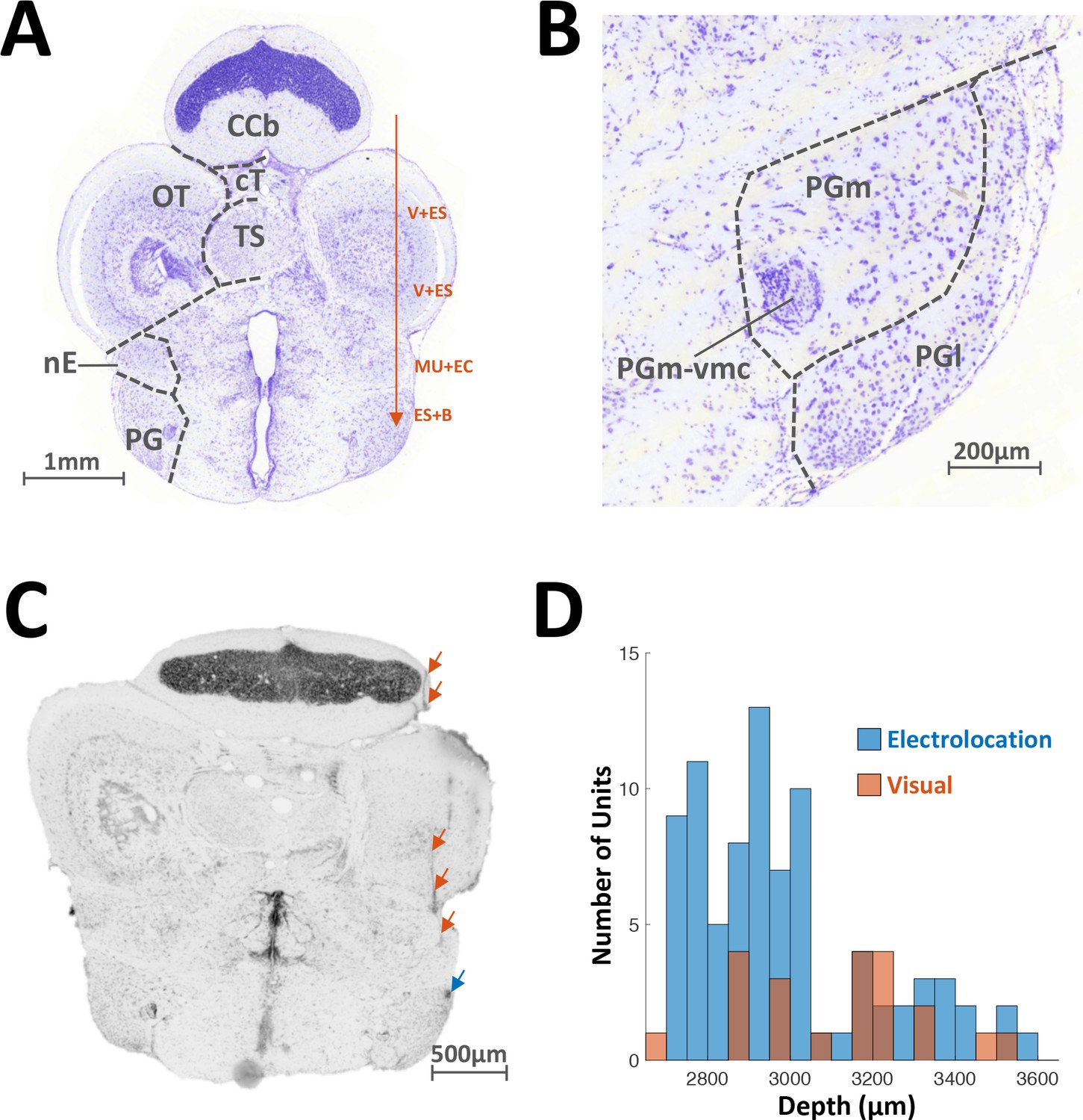
(A) Transverse slice of the brain of A. Leptorhynchus, about 300 μm caudal to the midbrain-telencephalon boundary (around electric fish atlas level T24, Maler et al., 1991). Electrodes were inserted 800–1000 μm lateral to midline and advanced ventrally (red arrow). Visual and electrosensory stimuli were presented as the electrode was lowered in order to identify PG. There was variation in the depth of the various responses encountered depending on the size and precise orientation of the fish. Typically, visual and electrosensory (V + ES) responses were encountered around 1200 μm and 1900 μm ventrally to the top of the corpus cerebellum (CCb), as the electrode passed through the rostral edge of the optic tectum (Bastian, 1982). Further down, weak multi-unit activity responding to electro-communication signals (MU + EC) was usually detected around 2300–2500 μm, as the electrode passed through n. electrosensorius (nE, Heiligenberg et al., 1991). Finally, preglomerular (PG) responses were predominantly electrosensory and were characterized by bursting (ES + B, see Figure 1B–C). TS: Torus Semicircularis; cT: tectal commissure. (B) Close-up image of panel (A) showing the lateral (PGl) and medial (PGm) subdivisions of PG. PGm-vmc: ventromedial cell group of PGm. (C) Transverse slice prepared after recording motion-sensitive PG cells. The electrode track is visible through the edge of the cerebellum, the bottom of OT and nE (red arrows). The electrode tip mark is visible in PGl (blue arrow). (D) Distribution of depths (relative to top of cerebellum) where electrosensory motion-responsive (blue) and visual-responsive (red) single-units were recorded from. The visual units were usually in the more ventral portion of PG. We note that the recording depths correspond to the anatomical definition of PG and encompass its full extent (Maler et al., 1991).
Figure 2 with 1 supplement
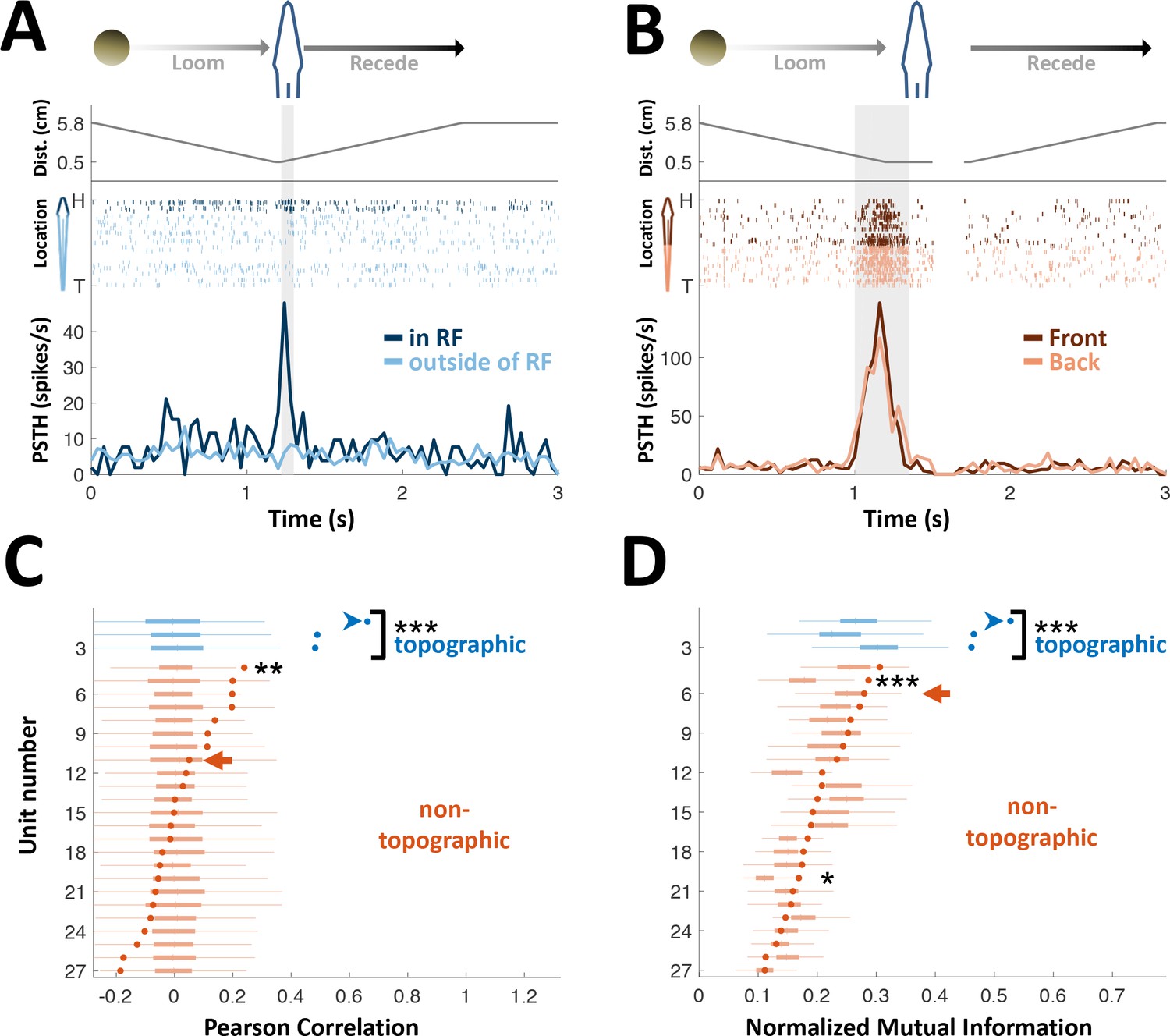
PG cells lack egocentric spatial information.
(A) Example of an ‘atypical’ topographic PG cell with a restricted receptive field (RF) at the head. Looming-receding motions were performed at different locations. Top: object distance from skin vs. time; middle: spike raster plot, arranged according to object location (H = head, T = tail); bottom: PSTH within the RF (dark blue) and outside of it (light blue). (B) Example of a ‘typical’ non-topographic PG cell, responding to stimulation across the entire body. Bottom: PSTH of front (dark red) and rear (light red) halves of fish. RF extended beyond the sampled range. (C) Circles: Pearson correlation between normalized egocentric location and firing-rate for all units, in ascending order; box-plots: distribution of correlations obtained by random permutations of locations (control). Only one non-topographic cell had correlations that statistically differed significantly from those in the randomized boxes (**). (D) Circles: normalized mutual information (MI) between egocentric location and firing-rate for all units, in ascending order; box plots, distribution of MI obtained by random permutations of locations (control). Only two non-topographic cells had MI that statistically differed significantly from those in the randomized boxes (* and ***). Blue arrowheads in (C) and (D) mark the cell depicted in (A); Red arrows mark the cell depicted in (B). P values obtained using permutation test: ‘*’, p < 0.05; ‘**’, p < 0.01; ‘***’, p < 0.001.
Figure 2—figure supplement 1
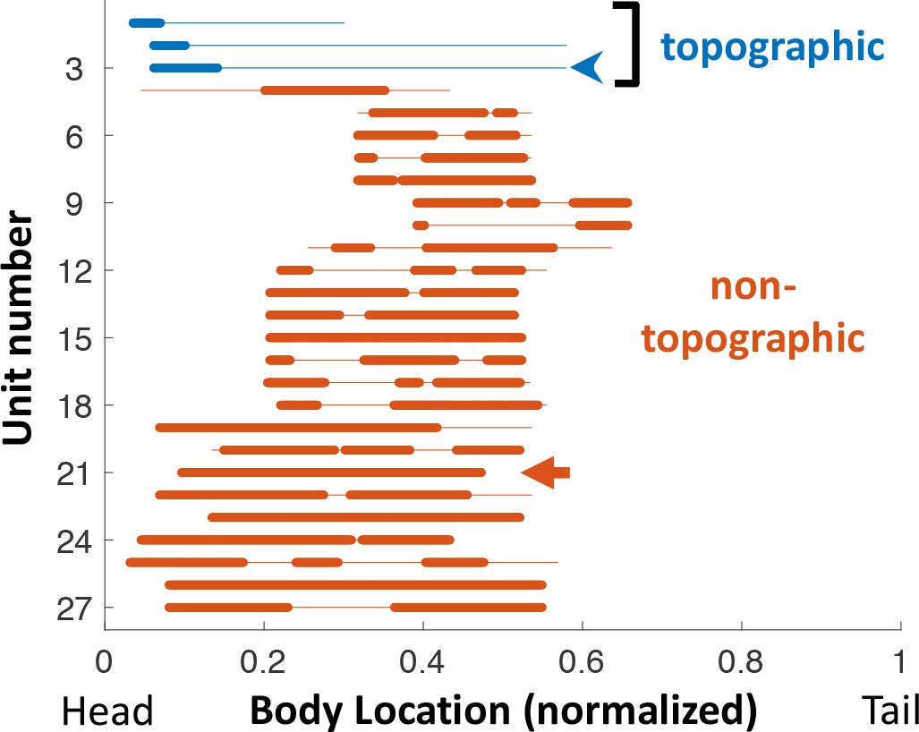
Receptive fields across the PG population.
Each line depicts the RF of one unit tested with the RF sampling protocol. Location along the body was normalized to total fish length. Thin line: range sampled (affected by the fish size and position within the tank); The hindmost third of the body was never sampled, as it has a very low density of electroreceptors (Carr et al., 1982) and is also too close to the electric organ. Thick line: positions in which unit’s response was statistically significant (see Materials and methods). Blue arrowhead: unit depicted in Figure 2A. Red arrow: unit depicted in Figure 2B. Note that for most units the RF extends beyond the sampled range. Also note that all three topographic units had RF at the rostral edge of the head, where electroreceptor density is maximal (Carr et al., 1982).
Figure 3 with 2 supplements
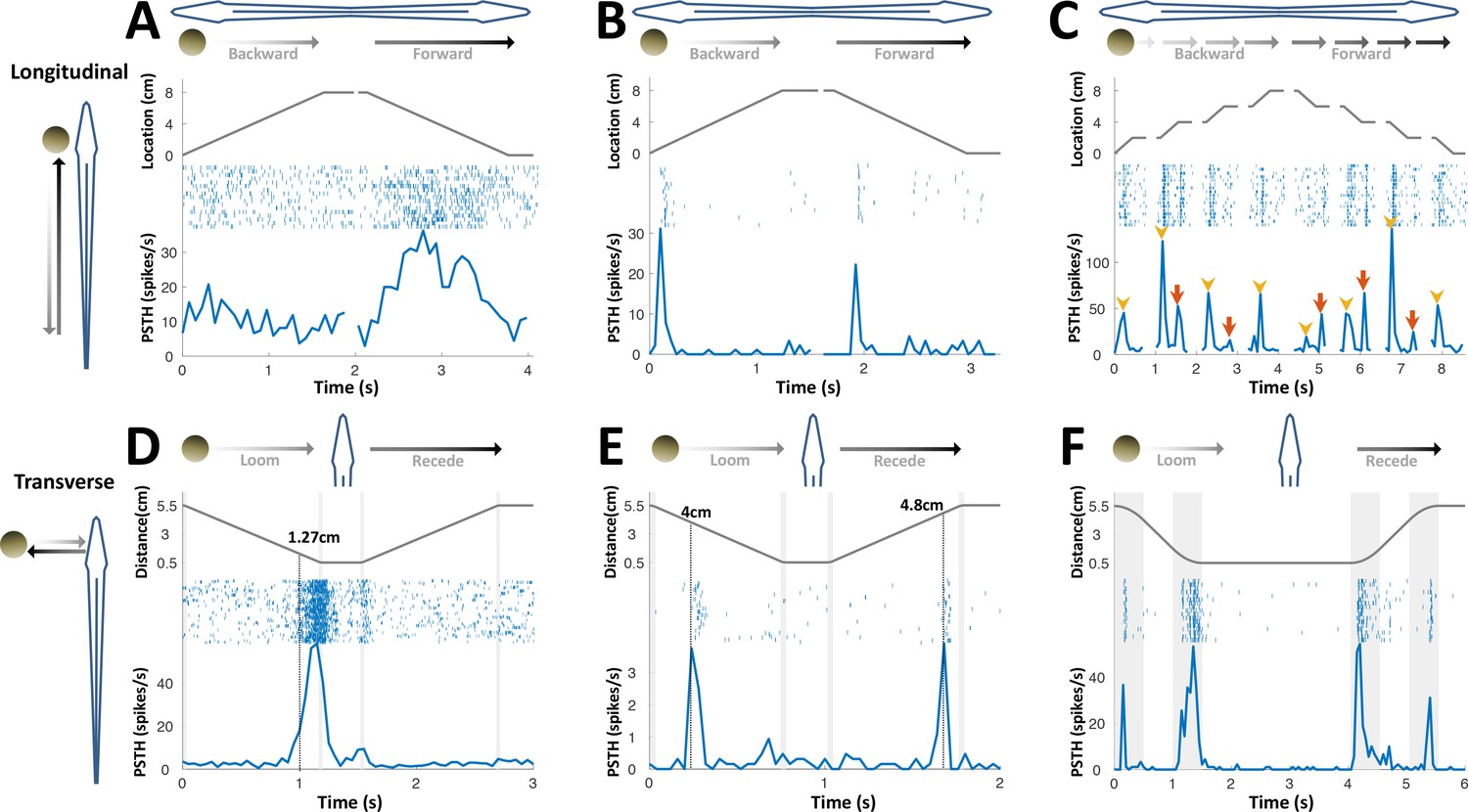
PG cells respond to motion novelty.
(A–C) Longitudinal motion. Top: object location (distance from the tip of the nose); middle: spike raster; bottom: PSTH. (A) ‘Atypical’ PG cell responding uni-directionally, throughout the motion toward the head. 43% (3/7) of atypical PG cells responded during forward motion only, while 57% (4/7) responded in both directions. (B) ‘Typical’ PG cell responding to motion-onset at the head during backward motion and to motion-onset at the tail during forward motion. 75% (15/20) of these motion novelty cells respond bi-directionally, 10% (2/20) only during forward motion and 15% (3/20) only during backward motion. (C) PG cell responding to motion onset (yellow arrowheads) and to motion offset (red arrows) in intermittent-motion protocol. (D–F) Responses to transverse (looming-receding) motion. All PG cells recorded with transverse-motion (40/40) responded to object looming, while only 40% (16/40) responded to receding. Top: object distance from skin; middle: spike raster; bottom: PSTH. Grey shadings mark acceleration/deceleration. (D) Proximity detector cell. Note that the response starts prior to the deceleration (shaded). (E) Encounter detector cell. (F) Motion change detector cell, responding when objects accelerated/decelerated (shaded, 10 cm/s2 in this example) similarly to the response observed to longitudinal motion (panels B and C).
Figure 3—figure supplement 1
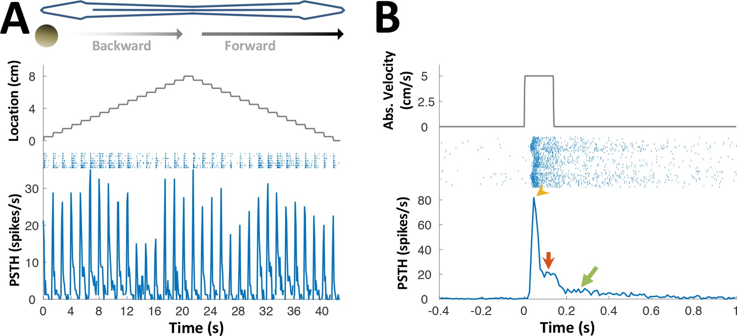
PG lateral-line responses.
Response of an example PG cell to longitudinal motion of an agar sphere (15% agarose dissolved in tank water). The sphere’s conductivity was identical to that of the surrounding water, making it electrically invisible (Heiligenberg, 1973). Acoustic stimuli were also delivered to exclude the possibility of an auditory response. The relatively small number of lateral-line sensitive cells found (N = 7) precludes systematic characterization of the response properties of these cells. (A) Motion in each direction was broken into 16 segments separated by wait period (similar to Figure 3C). The cell responded to this motion in either direction, anywhere across the body surface. Since the object was electrically invisible, these responses likely reflect activation of the lateral-line system, which was shown to project to PG (Giassi et al., 2012a). (B) Cell response, averaged across body locations. Top: absolute velocity (cm/s); middle: spike raster plot; bottom: PSTH. Note that unlike most electrosensory PG cells (see Figure 3), this cell displayed not only motion onset response (yellow arrowhead), but also a response to continuous motion (red arrow) and prolonged response after motion cessation (green arrow; this post-stimulus discharge likely reflects wave reverberations in the experimental tank). This continuous response mode suggests that lateral-line related activity in PG conveys swimming velocity information, which can then be combined in the pallium (DL) with the time-interval information reported here to produce allocentric distance estimation between objects.
Figure 3—figure supplement 2
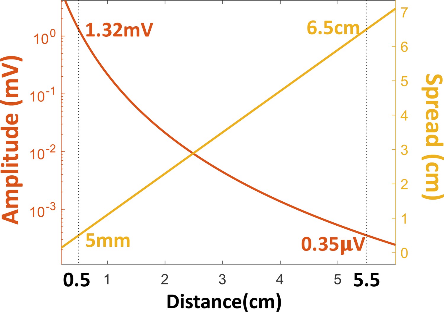
The amplitude (left ordinate, log scale) and spread (right ordinate, linear scale) of the object’s electric image on the skin, as functions of distance, based on a previously published model of electric fields in this fish (Chen et al., 2005).
https://doi.org/10.7554/eLife.36769.012
Figure 4
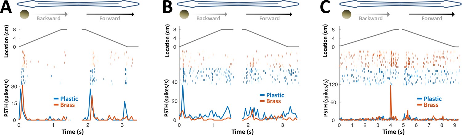
PG response to conductive/non-conductive objects.
(A–C) Top: object location (distance from the tip of the nose) during longitudinal object motion; middle: spike raster; bottom: PSTH. Red: conductive object (brass sphere, mimicking plants and animals); Blue: non-conductive object (plastic sphere, mimicking rocks). (A) Example cell responding to both brass and plastic spheres (such responses were found in 57% of the cells, 24/42). (B) Example cell responding primarily to plastic, with a very faint response to brass (5% of the cells, 2/42). (C) Example cell responding to brass only (38% of the cells, 16/42). The predominance of cells responding to both brass and plastic spheres or to brass-only spheres is likely inherited from OT (Bastian, 1982).
Figure 5 with 2 supplements
History-independent, spatially non-specific adaptation of PG cells.
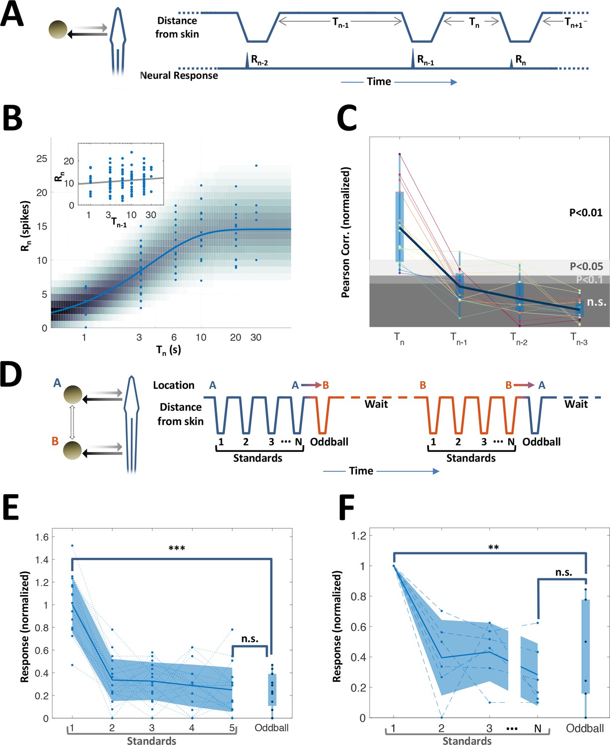
(A) Random interval protocol. Object motions toward- and away-from-skin generated responses , measured by spike count within individually determined time-window. Motions were interleaved by random time intervals (1–30 s). (B) Response versus the preceding time-interval (log scale) for an example neuron (circles). Model fitted to the data-points is depicted by response rate (solid blue line) and spike count distribution (background shading); correlation of data to model = 0.56 (p < 10−6, random permutations). Inset: same data-points plotted as function of penultimate intervals; grey line: linear regression to log(T) (correlation = 0.15, p = 0.136, random permutations). (C) Correlations between responses and time-intervals (last interval and one-, two- or three-before-last), normalized to the 10, 5 and 1 top percentiles of correlations generated by random permutations of the data, for each of the 15 adapting cells tested (thin colored lines; thick blue line: mean across population). For most cells, the response was significantly correlated only with the last interval. (D) Spatial oddball protocol. A sequence of N standard stimuli at one location (N = 5–9) was followed by one oddball stimulus at a different location. (E) Response of example cell (normalized to non-adapted response) to oddball protocol (dotted lines: individual tirals, N = 10; thick line and shaded area: mean ± standard deviation). Response to the oddball was significantly weaker than the non-adapted response (p < 10−4, bootstrap) and not significantly different from the response to the last standard stimulus (p = 0.45, bootstrap). (F) Normalized response of all adapting cells tested with the spatial oddball protocol (dashed lines: individual cells, N = 6; thick line and shaded area: mean ± standard deviation). Population response to the oddball was significantly weaker than the non-adapted response (p = 0.001, bootstrap) and not significantly different from response to the last standard stimulus (p = 0.2, bootstrap). ‘**’, p < 0.01; ‘***’, p < 0.001; n.s., not significant.
Figure 5—figure supplement 1
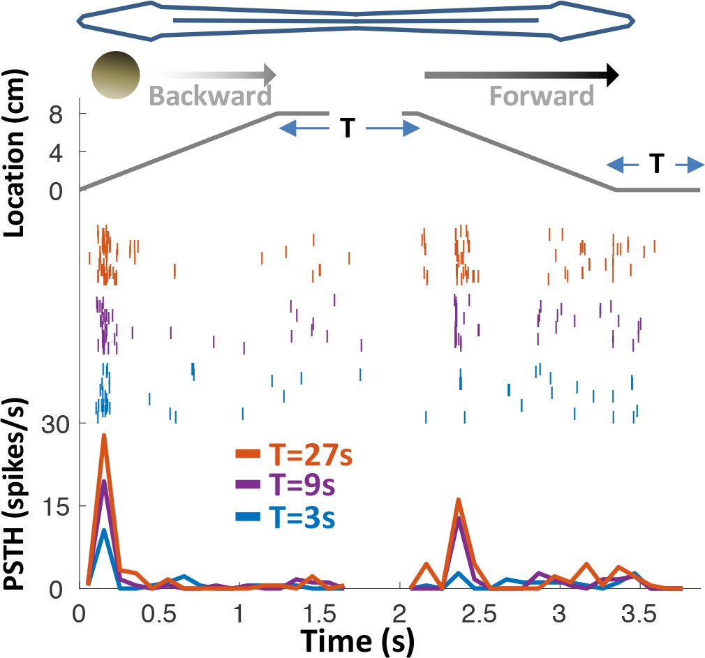
Response adaptation to periodic motion.
An example motion-onset responsive cell was stimulated with repetitive back-and-forth longitudinal motion. Duration of wait intervals between movements (T) was 3, 9 or 27 s (color-coded as blue, purple and red, respectively). Top: object position relative to head; middle: spike raster; bottom: PSTHs. 45% (15/33) of PG cells exhibited pronounced adaptation to repeated motion, with time-constants on the order of seconds to tens of seconds. In this example, the response strength for T = 27 s was larger than for T = 9 s, which in turn was larger than for T = 3 s – indicating a time-constant of adaptation >>1 s.
Figure 5—figure supplement 2

PG Visual responses.
(A) Response of an example PG cell to longitudinal motion of a light source. Note the strong onset and offset responses. (B) Circles: ON response (, total number of spikes during backward motion) of the cell depicted in panel A, as a function of the duration of the preceding time-interval (1-30 s). Dynamic adaptation model was fitted to the data (β=0 for this cell); solid blue line: response rate of model fitted to the data-points; background shading: spike count distribution of the model. ON response intensity of this cell is highly correlated with the duration of the last interval (correlation=0.467, P < 10−6, random permutations). Inset: same data-points plotted as function of penultimate intervals; grey line: linear regression to log(T) (correlation= –0.022, P = 0.75, random permutations). (C) Correlations between responses and time-intervals – for the last intervals and one-, two- or three-before last intervals (Tn, Tn-1, Tn-2, Tn-3), normalized to the significance level using random permutations, and plotted here for all the adapting visual cells that we recorded (n = 3). Only the last interval (Tn) was significantly correlated with the response of the cells – demonstrating that PG cells display history-independent adaptation in other modalities and not just the electrosensory one.
Figure 6 with 1 supplement
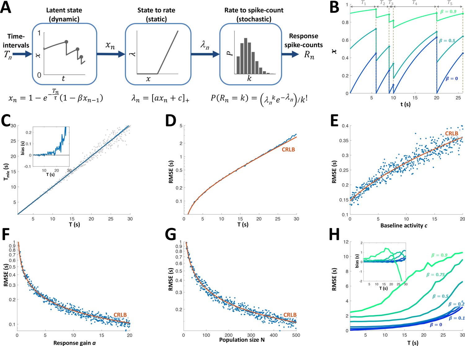
Adaptation model and Maximum Likelihood Estimation of time inteval (A) Block diagram of adaptation model, which includes three stages: a dynamic latent state variable with memory parameter and exponential recovery with time-constant ; a static non-negative mapping from state to firing parameter , with gain parameter a and baseline parameter c; and a stochastic spike-count generator (Poisson random variable with parameter ).
(B) Examples of state variable dynamics due to a random encounter sequence, for different values of . Note that when , each encounter entails complete reset of to 0, thus generating the history independence property. (C) MLE of time interval with a homogeneous population. Grey circles: individual estimations; blue curve: mean; black line: identity diagonal. Inset: estimation bias. (D) Blue: root-mean-squared estimation error (RMSE, log scale) vs. time interval. Red: Cramér-Rao Lower Bound (CRLB). (E) RMSE vs baseline activity c. (F) RMSE (log scale) vs. response gain a. (G) RMSE(log scale) vs. population size N. (H) RMSE for different values of . Inset: estimation bias. In all simulations unless stated otherwise.
Figure 6—figure supplement 1
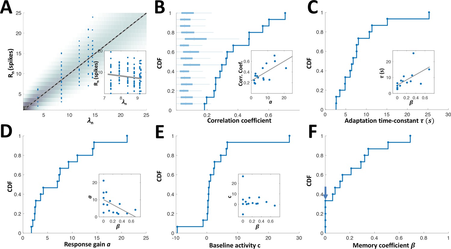
Empirical distributions of model parameters.
(A) Circles: measured responses of one example adapting cell, plotted against the response rates of the model for this cell (computed from the interval sequence using equations (1) and (2) in Methods); background shading: spike count distribution of the model; solid grey line: linear regression (Pearson’s correlation: 0.706, p < 10−4 random permutations); dashed black line: identity diagonal. Inset: responses vs. rates for example non-adapting cell (Pearson’s correlation: -0.14, p = 0.123 random permutations). (B) Cumulative distribution function (CDF) of Pearson’s correlation coefficient between the measured responses and the response rate of the fitted model. Correlations for all adapting cells were statistically significant (P < 0.05, random permutations); box-plots: distributions of correlations (absolute value), obtained by random permutations of responses of each cell. Inset: the correlation coefficient strongly depended on the response gain a; high gain neurons yielded the strongest correlations. Grey line: linear regression. (C) CDF of adaptation time-constant . Inset: cells with high values of had longer time-constants (Pearson’s correlation 0.594, p = 0.019). (D) CDF of response gain parameter a. Inset: cells with low values of had higher gain (Pearson’s correlation -0.532, p = 0.04), that is the history-independent cells provide more precise temporal representation (see Figure 6F). (E) CDF of baseline activity parameter c. Negative values were obtained for units with high threshold, that is that stopped responding altogether at short time intervals. Inset: baseline activity was not significantly correlated with (Pearson’s correlation -0.15, p=0.593). (F) CDF of memory parameter . Note that 33% (5/15) of the cells were best fitted with (arrow).
Figure 7
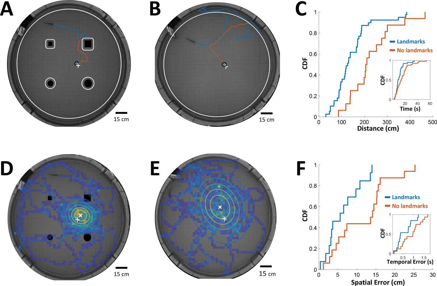
Path integration accuracy measured in behaving fish.
(A) Fish navigating to food placed at designated location (white ‘+’ sign) with the aid of landmarks (black silhouettes). Orange line: cruising distance from the last encounter (3 cm from landmark or 6 cm from wall, white contours) to the detection of the food (3 cm from food, black contour around white ‘+’ sign). (B) Same as A in an experiment with no landmarks. Note the increase in traveled path. (C) Cumulative distribution functions (CDF) of the distances from last encounter to food, with (blue) and without (red) landmarks. Inset: CDFs of time elapsed from last encounter to food. (D) Fish searching for missing food in a probe trial with landmarks. Heat map: visit histogram; colored ovals: 2-D Gaussian fitting of histogram; the spatial error is the distance from fitted Gaussian center (white ‘x’) to the memorized food location (white ‘+’). (E) Probe trial without landmarks. Note the increase in error compared with panel D. (F) Cumulative distribution functions (CDF) of the fish’s spatial errors, with (blue) and without (red) landmarks. Inset: CDFs of the temporal errors, obtained by dividing the spatial errors by the fish’s average velocity.
Figure 8
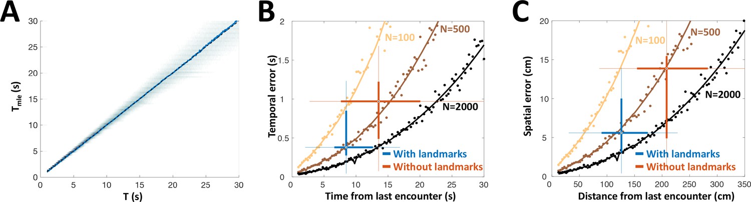
PG simulation explains animals’ spatial and temporal behavioral accuracy.
(A) Distribution of estimated time interval vs. actual time interval using a heterogeneous population (N = 500 cells). Estimation is approximately unbiased: the mean (blue line) follows the identity diagonal. (B) Temporal representation. Circles: mean error obtained numerically with 100 (yellow), 500 (brown) and 2000 (black) cells. Curves: CRLB computed analytically. Two-dimensional boxplots: distribution of behavioral temporal estimation errors vs. time from last encounter (blue: with landmarks, red: without landmarks, see Figure 7). (C) Spatial representation. MLE temporal results were converted to distance by multiplying by the median velocity reported for navigating fish (12 cm/s) (Jun et al., 2016).
Additional files
-
Transparent reporting form
- https://doi.org/10.7554/eLife.36769.021
Download links
A two-part list of links to download the article, or parts of the article, in various formats.
Downloads (link to download the article as PDF)
Open citations (links to open the citations from this article in various online reference manager services)
Cite this article (links to download the citations from this article in formats compatible with various reference manager tools)
A time-stamp mechanism may provide temporal information necessary for egocentric to allocentric spatial transformations
eLife 7:e36769.
https://doi.org/10.7554/eLife.36769


