Persistent coding of outcome-predictive cue features in the rat nucleus accumbens
- Dartmouth College, United States
Figures
Figure 1
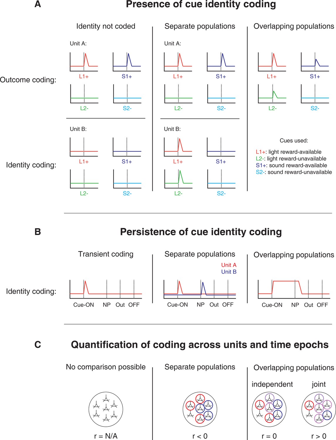
Schematic of hypothetical coding scenarios for cue feature coding employed by single units in the NAc across different cue features (A) and phases of a trial (B).
(A) Schematic peri-event time histograms (PETHs) illustrating putative responses to different cues under different hypotheses of how cue identity (light, sound; L, S) and outcome (reward-available, reward-unavailable; +, -) are coded. Left panel: Coding of identity is absent in the NAc. Top: Unit A encodes a motivationally relevant variable, such as expected outcome, similarly across other cue features, such as identity or physical location. Hypothetical plot is firing rate across time. L1+ (red) signifies a reward-available light cue, S1+ (navy blue) a reward-available sound cue, L2- (green) a reward-unavailable light cue, S2- (light blue) a reward-unavailable sound cue. Dashed line indicates onset of cue. Bottom: No units within the NAc discriminate their firing according to cue identity. Middle panel: Coding of identity occurs in a separate population of units from coding of other cue features such as expected outcome or physical location. Top: Same as left panel, with unit A discriminating between reward-available and reward-unavailable cues. Bottom: Unit B discriminates firing across stimulus modalities, depicted here as firing to light cues but not sound cues. Note lack of coding overlap in both units. Right panel: Coding of identity occurs in an overlapping population of cells with coding of other motivationally relevant variables. Hypothetical example demonstrating a unit that responds to reward-available cues, but firing rate is also modulated by the stimulus modality of the cue, firing most for the reward-available light cue. (B) Schematic PETHs illustrating potential ways in which identity coding may persist over time. Left panel: Cue-onset triggers a transient response to a unit that codes for cue identity. Dashed lines indicate time of a behavioural or environmental event. 'Cue-ON’ signifies cue-onset, 'NP’ signifies nosepoke at a reward receptacle, 'Out’ signifies when the outcome is revealed, 'OFF’ signifies cue-offset. Middle and right panel: Identity coding persists at other time points, shown here during a nosepoke hold period until outcome is revealed. Coding can either be maintained by a sequence of units (middle panel) or by the same unit as during cue-onset (right panel). (C) Schematic pool of NAc units, illustrating different analysis outcomes that discriminate between hypotheses. R values represent the correlation between sets of recoded regression coefficients (see text for analysis details). Left panel: Cue identity is not coded (A: left panel), or is only transiently represented in response to the cue (B: left panel). Middle panel: Negative correlation (r < 0) suggests that identity and outcome coding are represented by separate populations of units (A: middle panel), or identity coding is represented by distinct units across different points in a trial (B: middle panel). Red circles represents coding for one cue feature or point in time, blue circles for the other cue feature or point in time. Right panel: Identity and outcome coding (A: right panel), or identity coding at cue-onset and nosepoke (B: right panel) are represented by overlapping populations of units, shown here by the purple circles. The absence of a correlation (r = 0) suggests that the overlap of identity and outcome coding, or identity coding at cue-onset and nosepoke, is expected by chance and that the two cue features, or points in time, are coded by overlapping but independent populations from one another. A positive correlation (r > 0) implies a higher overlap than expected by chance, suggesting coding by a joint population. Note: The same logic applies to other aspects of the environment when the cue is presented, such as the physical location of the cue, as well as other time epochs within the task, such as when the animal receives feedback about an approach.
Figure 2
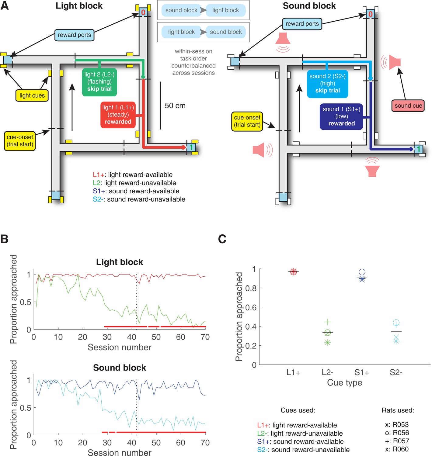
Schematic and performance of the behavioural task.
(A) Apparatus was a square track consisting of multiple identical T-choice points. At each choice point, the availability of 12% sucrose reward at the nearest reward receptacle (light blue fill) was signalled by one of four possible cues, presented when the rat initiated a trial by crossing a photobeam on the track (dashed lines). Photobeams at the ends of the arms by the receptacles registered nosepokes. Arrows outside of track indicate correct running direction. Left: light block showing an example trajectory for a correct reward-available (approach trial; red) and reward-unavailable (skip trial; green) trial. Rectangular boxes with yellow fill indicate location of LEDs used for light cues. Right: sound block with a correct reward-available (approach trial; navy blue) and reward-unavailable (skip trial; light blue) trial. Speakers for sound cues were placed underneath the choice points, indicated by magenta speaker icons. Ordering of the light and sound blocks was counterbalanced across sessions. Reward-available and reward-unavailable cues were presented pseudo-randomly, such that not more than two of the same type of cue could be presented in a row. Location of the cue on the track was irrelevant for behaviour, all cue locations contained an equal amount of reward-available and reward-unavailable trials. (B-C) Performance on the behavioural task. B. Example learning curves across sessions from a single subject (R060) showing the proportion of trials approached for reward-available (red line for light block, navy blue line for sound block) and reward-unavailable trials (green line for light block, light blue line for sound block) for light (top) and sound (bottom) blocks. Fully correct performance corresponds to an approach proportion of 1 for reward-available trials and 0 for reward-unavailable trials. Rats initially approach on both reward-available and reward-unavailable trials, and learn with experience to skip reward-unavailable trials. Red bars indicate days in which a rat statistically discriminated between reward-available and reward-unavailable cues, determined by a chi square test. Dashed line indicates time of electrode implant surgery. (C) Proportion of trials approached for each cue, averaged across all recording sessions and shown for each rat. Different columns indicate the different cues (reward-available (red) and reward-unavailable (green) light cues, reward-available (navy blue) and reward-unavailable (light blue) sound cues). Different symbols correspond to individual subjects; horizontal black line shows the mean. All rats learned to discriminate between reward-available and reward-unavailable cues, as indicated by the clear difference of proportion approached between reward-available (90% approached) and reward-unavailable cues (30% approached), for both blocks (see Results for statistics).
Figure 3 with 2 supplements
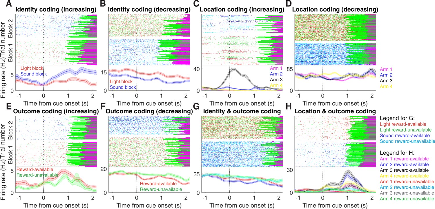
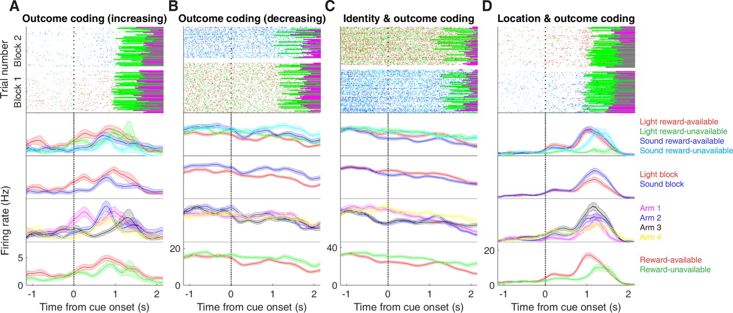
Examples of cue-modulated NAc units influenced by different task parameters.
(A) Example of a cue-modulated NAc unit that showed an increase in firing following the cue, and exhibited identity coding. Top: raster plot showing the spiking activity across all trials aligned to cue-onset. Spikes across trials are colour-coded according to cue type (red: reward-available light; green: reward-unavailable light; navy blue: reward-available sound; light blue: reward-unavailable sound). Green and magenta bars indicate trial termination when a rat initiated the next trial or made a nosepoke, respectively. White space halfway up the raster plot indicates switching from one block to the next. Dashed line indicates cue-onset. Bottom: PETHs showing the average smoothed firing rate for the unit for trials during light (red) and sound (blue) blocks, aligned to cue-onset. Lightly shaded area indicates standard error of the mean. Note this unit showed a larger increase in firing to sound cues. (B) An example of a unit that was responsive to cue identity as in A, but for a unit that showed a decrease in firing to the cue. Note the sustained higher firing rate during the light block. (C-D) Cue-modulated units that exhibited location coding. Each colour in the PETHs represents average firing response for a different cue location. (C) The firing rate of this unit only changed on arm 3 of the task. (D) Firing rate decreased for this unit on all arms but arm 4. (E-F) Cue-modulated units that exhibited outcome coding, with the PETHs comparing reward-available (red) and reward-unavailable (green) trials. (E) This unit showed a slightly higher response during presentation of reward-available cues. (F) This unit showed a dip in firing when presented with reward-available cues. (G-H) Examples of cue-modulated units that encoded multiple cue features. (G) This unit showed both identity and outcome coding. (H) An example of a unit that coded for both identity and location.
Figure 3—figure supplement 1
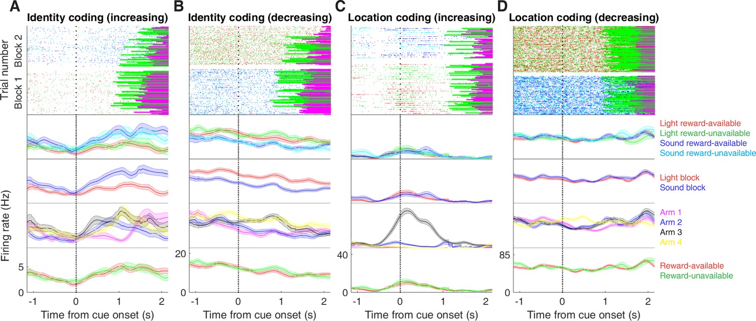
Expanded examples of cue-modulated NAc units influenced by different task parameters for Figure 3A–D, showing firing rate breakdown by: cue type (top PETH), cue identity (top-middle PETH), cue location (bottom-middle PETH), and cue outcome (bottom PETH).
https://doi.org/10.7554/eLife.37275.005
Figure 3—figure supplement 2
Expanded examples of cue-modulated NAc units influenced by different task parameters for Figure 3E–H, showing firing rate breakdown by: cue type (top PETH), cue identity (top-middle PETH), cue location (bottom-middle PETH), and cue outcome (bottom PETH).
https://doi.org/10.7554/eLife.37275.006
Figure 4 with 2 supplements
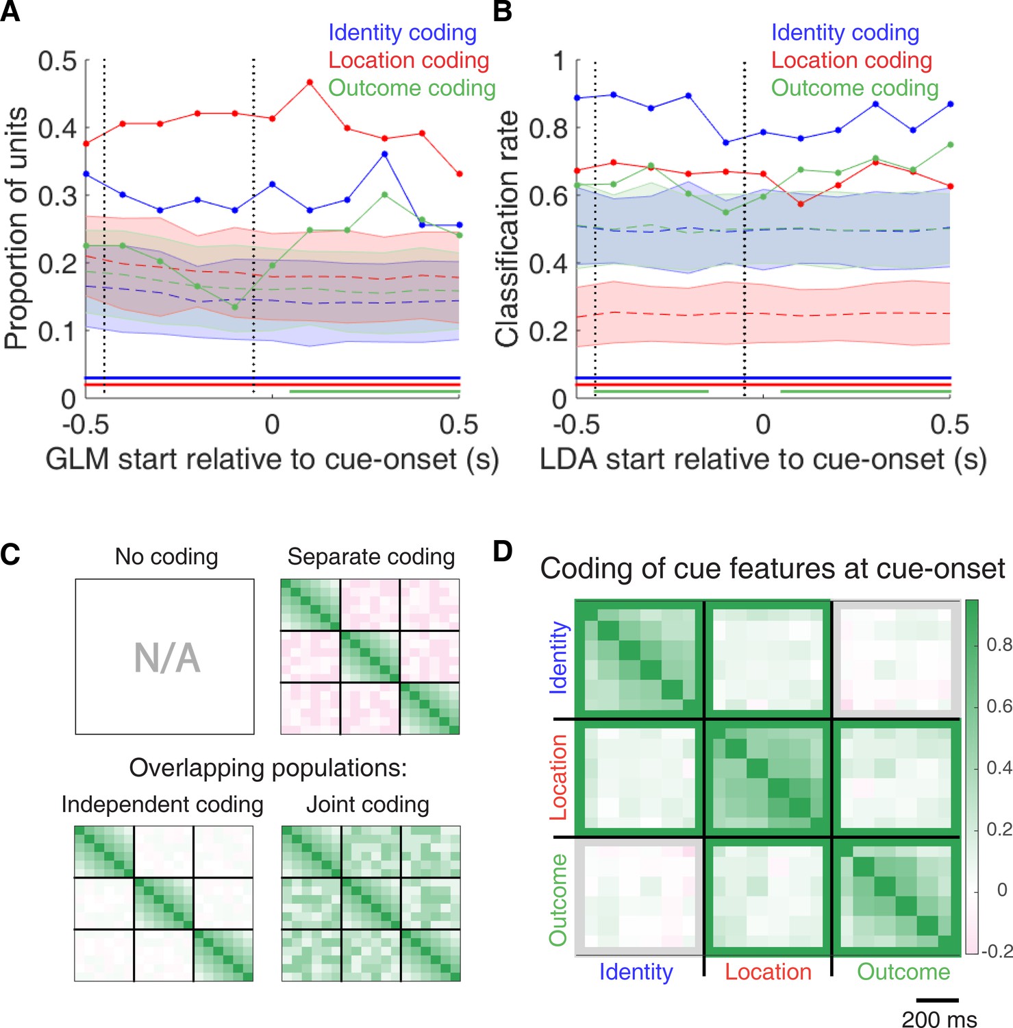
Summary of influence of cue features on cue-modulated NAc units at time points surrounding cue-onset.
(A) Sliding window GLM (bin size: 500 ms; step size: 100 ms) demonstrating the proportion of cue-modulated units where cue identity (blue solid line), location (red solid line), and outcome (green solid line) significantly contributed to the model at various time epochs relative to cue-onset. Dashed coloured lines indicate the average of shuffling the firing rate order that went into the GLM 100 times. Error bars indicate 1.96 standard deviations from the shuffled mean. Solid lines at the bottom indicate when the proportion of units observed was greater than the shuffled distribution (z-score > 1.96). Points in between the two vertical dashed lines indicate bins where both pre- and post-cue-onset time periods were used in the GLM. (B) Sliding window LDA (bin size: 500 ms; step size: 100 ms) demonstrating the classification rate for cue identity (blue solid line), location (red solid line), and outcome (green solid line) using a pseudoensemble consisting of the 133 cue-modulated units. Dashed coloured lines indicate the average of shuffling the firing rate order that went into the cross-validated LDA 100 times. Solid lines at the bottom indicate when the classifier performance greater than the shuffled distribution (z-score > 1.96). Points in between the two vertical dashed lines indicate bins where both pre- and post-cue-onset time periods were used in the classifier. (C-D) Correlation matrices testing the presence and overlap of cue feature coding at cue-onset. (C) Schematic outlining the possible outcomes for coding across cue features at cue-onset, generated by correlating the recoded beta coefficients from the GLMs and comparing to a shuffled distribution (see text for analysis details). Top left: coding is not present, therefore no comparison is possible. Top right: cue features are coded by separate populations of units. Displayed is a correlation matrix with each of the nine blocks representing correlations for two cue features across the post-cue-onset time bins from the sliding window GLM, with green representing positive correlations (r > 0), pink representing negative correlations (r < 0), and white representing no correlation (r = 0). X- and y-axis have the same axis labels, therefore the diagonal represents the correlation of a cue feature against itself at that particular time point (r = 1). Here the large amount of pink in the off-diagonal elements suggests that coding of cue features occur separately from one another. Bottom left: Coding of cue features occurs in overlapping but independent populations of units, shown here by the abundance of white and relative lack of green and pink in the off-diagonal elements. Bottom right: Coding of cue features occurs in a joint (correlated) overlapping population, shown here by the large amount of green in the off-diagonal elements. (D) Correlation matrix showing the correlation among cue identity, location, and outcome coding surrounding cue-onset. The window of GLMs used in each block is from cue-onset to the 500 ms window post-cue-onset, in 100 ms steps. Each individual value is for a sliding window GLM within that range, with the scale bar contextualizing step size. Colour bar displays relationship between correlation value and colour. Coloured square borders around each block indicate the result of a comparison of the mean correlation of a block to a shuffled distribution, with pink indicating separate populations (z-score < −1.96), grey indicating overlapping but independent populations, and green indicating joint overlapping populations (z-score > 1.96).
Figure 4—figure supplement 1
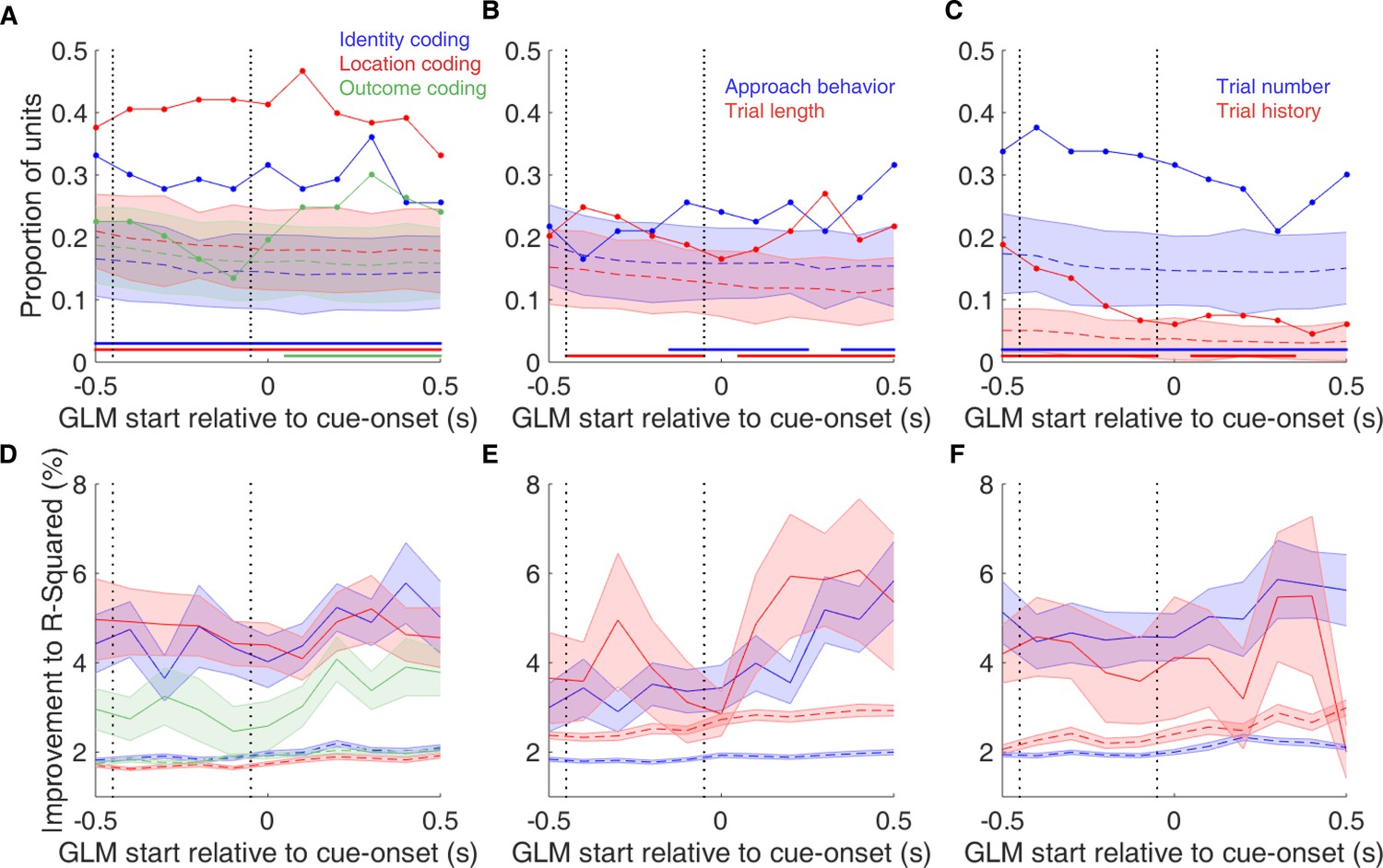
Summary of influence of various task parameters on cue-modulated NAc units at time points surrounding cue-onset.
(A-C) Sliding window GLM illustrating the proportion of cue-modulated units influenced by various predictors around time of cue-onset. (A) Sliding window GLM (bin size: 500 ms; step size: 100 ms) demonstrating the proportion of cue-modulated units where cue identity (blue solid line), location (red solid line), and outcome (green solid line) significantly contributed to the model at various time epochs relative to cue-onset. Dashed coloured lines indicate the average of shuffling the firing rate order that went into the GLM 100 times. Error bars indicate 1.96 standard deviations from the shuffled mean. Solid lines at the bottom indicate when the proportion of units observed was greater than the shuffled distribution (z-score > 1.96). Points in between the two vertical dashed lines indicate bins where both pre- and post-cue-onset time periods were used in the GLM. (B) Same as A, but for approach behaviour and trial length. (C) Same as A, but for trial number and trial history. (D-F) Average improvement to model fit. (D) Average percent improvement to R-squared for units where cue identity, location, or outcome were significant contributors to the final model for time epochs surrounding cue-onset. Shaded area around mean represents the standard error of the mean. (E) Same as D, but for approach behaviour and trial length. (F) Same D, but for trial number and trial history.
Figure 4—figure supplement 2
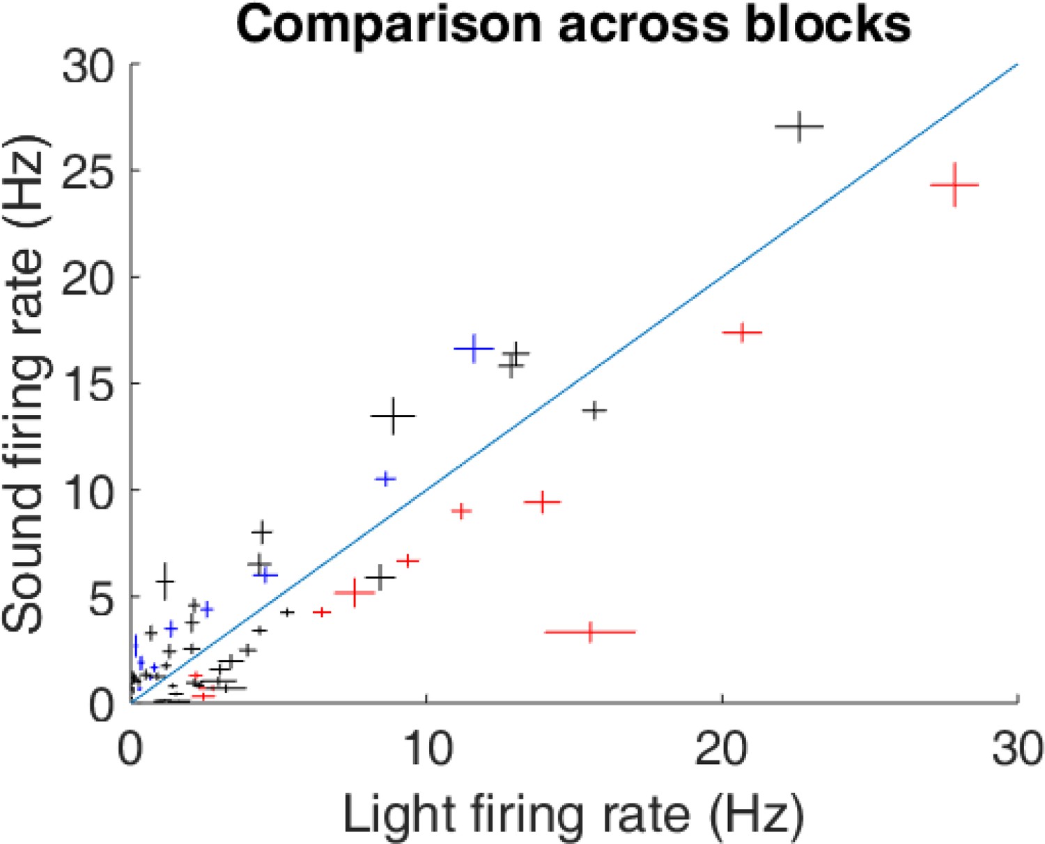
Scatter plot depicting comparison of firing rates for cue-modulated units across light and sound blocks.
Crosses are centered on the mean firing rate, range represents the standard error of the mean. Coloured crosses represents units that had cue identity as a significant predictor of firing rate variance in the GLM centered at cue-onset (blue are sound block preferring, red are light block preferring), whereas black crosses represent units where cue identity was not a significant predictor of firing rate variance. Diagonal dashed line indicates point of equal firing across blocks.
Figure 5 with 1 supplement
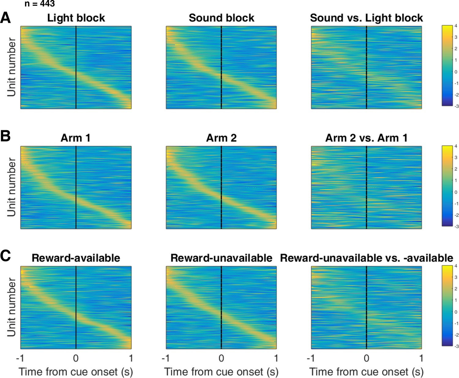
Distribution of NAc firing rates across time surrounding cue-onset.
Each panel shows normalized (z-score) peak firing rates for all recorded NAc units (each row corresponds to one unit) as a function of time (time 0 indicates cue-onset), averaged across all trials for a specific cue type, indicated by text labels. (A) left: Heat plot showing smoothed normalized firing activity of all recorded NAc units ordered according to the time of their peak firing rate during the light block. Each row is a unit’s average activity across time to the light block. Dashed line indicates cue-onset. Notice the yellow band across time, indicating all aspects of visualized task space were captured by the peak firing rates of various units. (A) middle: Same units ordered according to the time of the peak firing rate during the sound block. Note that for both blocks, units tile time approximately uniformly with a clear diagonal of elevated firing rates. (A) right: Unit firing rates taken from the sound block, ordered according to peak firing rate taken from the light block. Note that a weaker but still discernible diagonal persists, indicating partial similarity between firing rates in the two blocks. Colour bar displays relationship between z-score and colour. (B) Same layout as in A, except that the panels now compare two different locations on the track instead of two cue modalities. As for the different cue modalities, NAc units clearly discriminate between locations, but also maintain some similarity across locations, as evident from the visible diagonal in the right panel. Two example locations were used for display purposes; other location pairs showed a similar pattern. (C) Same layout as in A, except that panels now compare reward-available and reward-unavailable trials. Overall, NAc units coded experience on the task, as opposed to being confined to specific task events only. Units from all sessions and animals were pooled for this analysis.
Figure 5—figure supplement 1
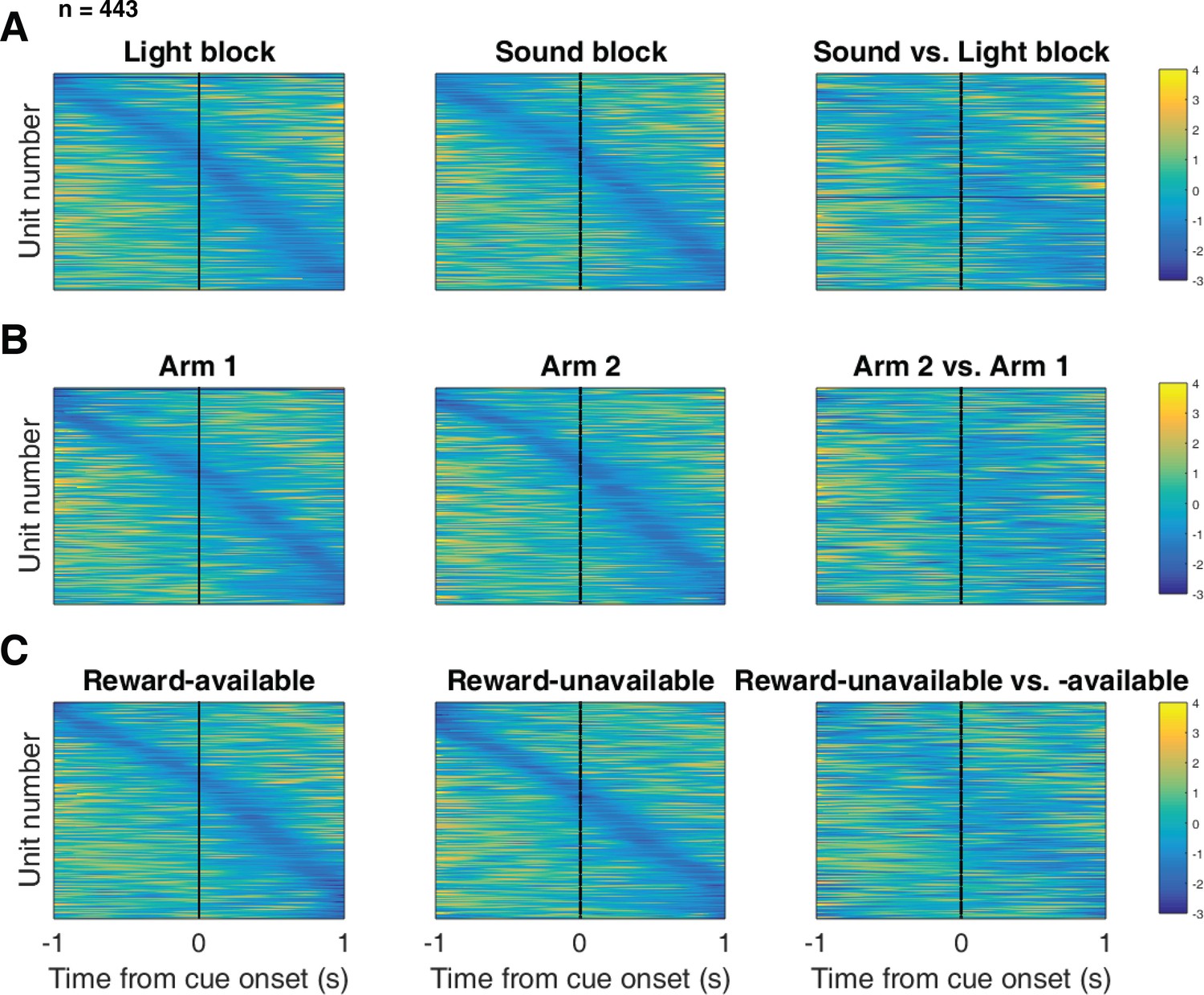
Distribution of NAc firing rates across time surrounding cue-onset.
Each panel shows normalized (z-score) minimum firing rates for all recorded NAc units (each row corresponds to one unit) as a function of time (time 0 indicates cue-onset), averaged across all trials for a specific cue type, indicated by text labels. (A) Responses during different stimulus blocks as in Figure 5A, but with units ordered according to the time of their minimum firing rate. (B) Responses during trials on different arms as in Figure 5B, but with units ordered by their minimum firing rate. (C) Responses during cues signalling different outcomes as in Figure 5C, but with units ordered by their minimum firing rate. Overall, NAc units coded experience on the task, as opposed to being confined to specific task events only. Units from all sessions and animals were pooled for this analysis.
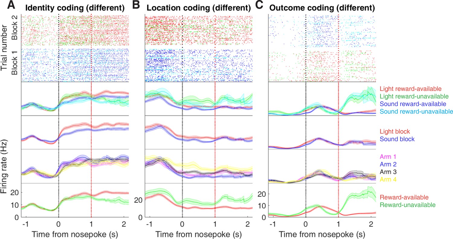
Figure 6 with 2 supplements
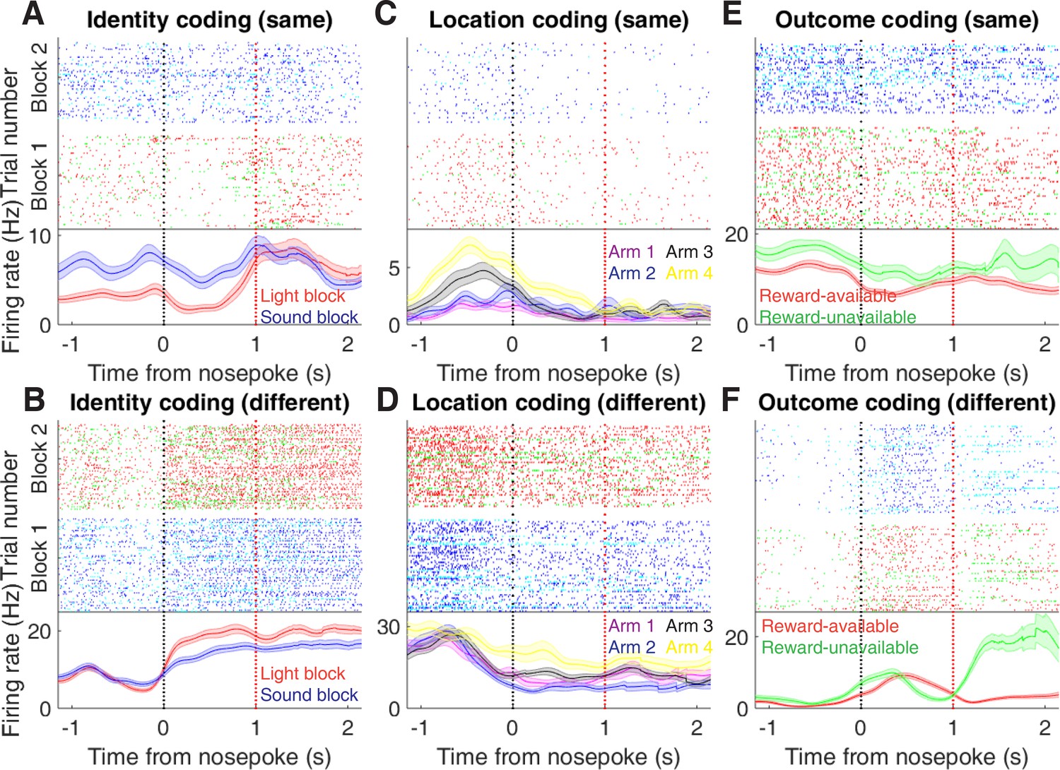
Examples of cue-modulated NAc units influenced by cue features at time of nosepoke.
(A) Example of a cue-modulated NAc unit that exhibited identity coding at both cue-onset and during subsequent nosepoke hold. Top: raster plot showing the spiking activity across all trials aligned to nosepoke. Spikes across trials are colour coded according to cue type (red: reward-available light; green: reward-unavailable light; navy blue: reward-available sound; light blue: reward-unavailable sound). White space halfway up the raster plot indicates switching from one block to the next. Black dashed line indicates nosepoke. Red dashed line indicates receipt of outcome. Bottom: PETHs showing the average smoothed firing rate for the unit for trials during light (red) and sound (blue) blocks, aligned to nosepoke. Lightly shaded area indicates standard error of the mean. Note this unit showed a sustained increase in firing to sound cues during the trial. (B) An example of a unit that was responsive to cue identity at time of nosepoke but not cue-onset. (C-D) Cue-modulated units that exhibited location coding, at both cue-onset and nosepoke (C), and only nosepoke (D). Each colour in the PETHs represents average firing response for a different cue location. (E-F) Cue-modulated units that exhibited outcome coding, at both cue-onset and nosepoke (E), and only nosepoke (F), with the PETHs comparing reward-available (red) and reward-unavailable (green) trials.
Figure 6—figure supplement 1
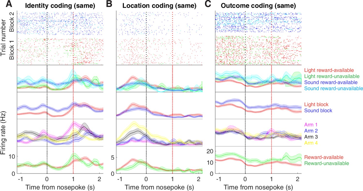
Expanded examples of cue-modulated NAc units influenced by different cue features at both cue-onset and during subsequent nosepoke hold for Figure 6A,C,E, showing firing rate breakdown by: cue type (top PETH), cue identity (top-middle PETH), cue location (bottom-middle PETH), and cue outcome (bottom PETH).
https://doi.org/10.7554/eLife.37275.014
Figure 6—figure supplement 2
Expanded examples of cue-modulated NAc units influenced by different cue features at time of nosepoke for Figure 6B,D,F, showing firing rate breakdown by: cue type (top PETH), cue identity (top-middle PETH), cue location (bottom-middle PETH), and cue outcome (bottom PETH).
https://doi.org/10.7554/eLife.37275.015
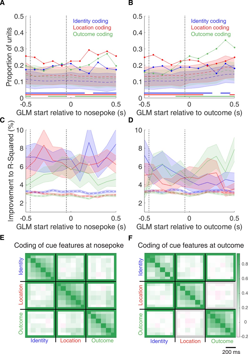
Figure 7 with 2 supplements
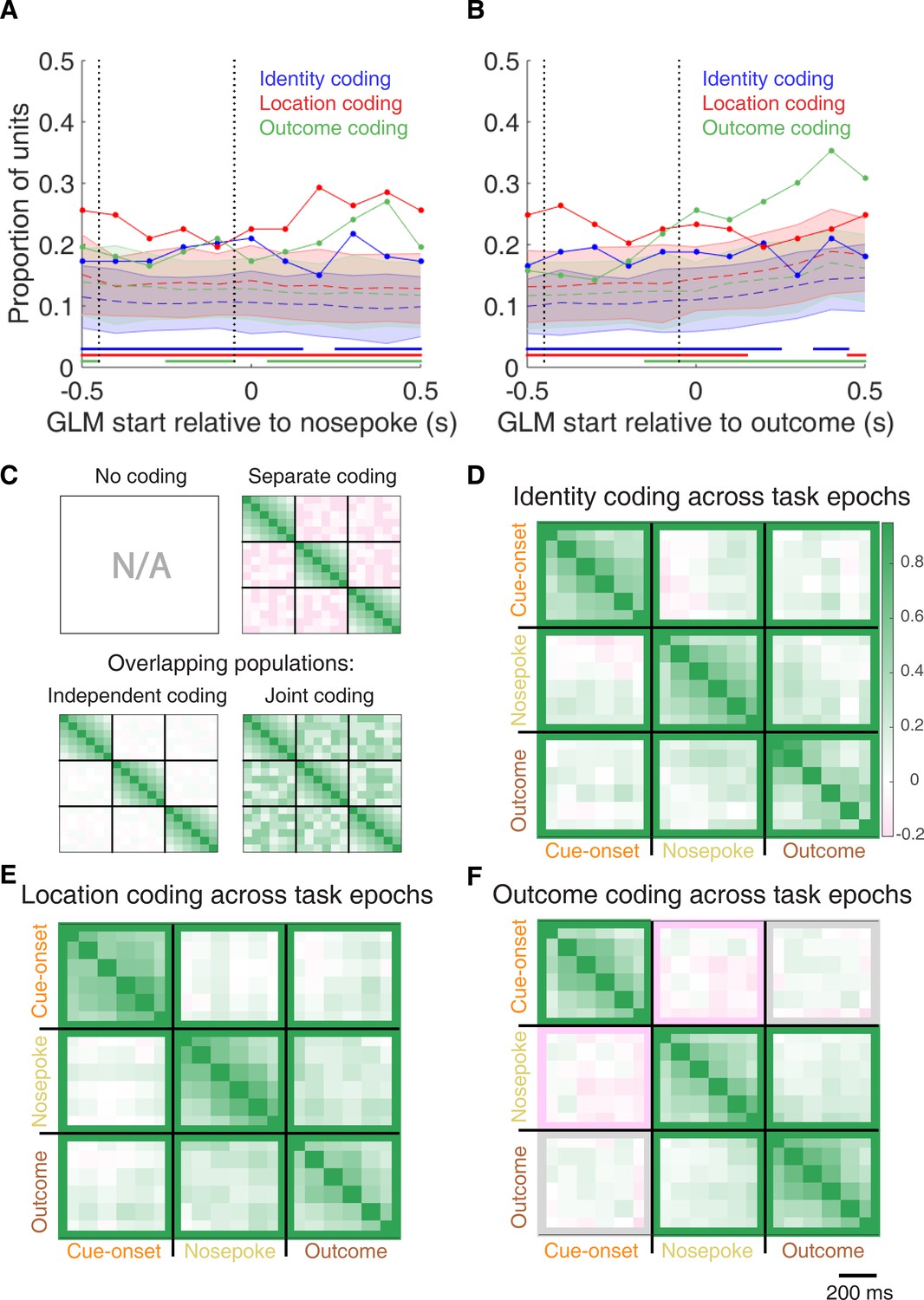
Summary of influence of cue features on cue-modulated NAc units at time points surrounding nosepoke and subsequent receipt of outcome.
(A-B) Sliding window GLM illustrating the proportion of cue-modulated units influenced by various predictors around time of nosepoke (A), and outcome (B). (A) Sliding window GLM (bin size: 500 ms; step size: 100 ms) demonstrating the proportion of cue-modulated units where cue identity (blue solid line), location (red solid line), and outcome (green solid line) significantly contributed to the model at various time epochs relative to when the rat made a nosepoke. Dashed coloured lines indicate the average of shuffling the firing rate order that went into the GLM 100 times. Error bars indicate 1.96 standard deviations from the shuffled mean. Solid lines at the bottom indicate when the proportion of units observed was greater than the shuffled distribution (z-score > 1.96). Points in between the two vertical dashed lines indicate bins where both pre- and post-cue-onset time periods were used in the GLM. (B) Same as A, but for time epochs relative to receipt of outcome after the rat got feedback about his approach. (C-F) Correlation matrices testing the persistence of cue feature coding across points in time. (C) Schematic outlining the possible outcomes for coding of a cue feature across various points in a trial, generated by correlating the recoded beta coefficients from the GLMs and comparing to a shuffled distribution (see text for analysis details). Top left: coding is not present, therefore no comparison is possible. Top right: a cue feature is coded by separate populations of units across time. Displayed is a correlation matrix with each of the nine blocks representing correlations for a cue feature across time bins for two task events from the sliding window GLM, with green representing positive correlations (r > 0), pink negative correlations (r < 0), and white representing significant correlation (r = 0). X- and y-axis have the same axis labels, therefore the diagonal represents the correlation of cue feature against itself at that particular time point (r = 1). Here the large amount of pink in the off-diagonal elements suggests that coding of a cue feature is accomplished by separate populations of units across time. Bottom left: Coding of a cue feature across time occurs in overlapping but independent populations of units, shown here by the abundance of white and relative lack of green and pink in the off-diagonal elements. Bottom right: Coding of a cue feature across time occurs in a joint overlapping population, shown here by the large amount of green in the off-diagonal elements. (D) Correlation matrix showing the correlation of units that exhibited identity coding across time points after cue-onset, nosepoke, and outcome receipt. The window of GLMs used in each block is from the onset of the task phase to the 500 ms window post-onset, in 100 ms steps. Each individual value is for a sliding window GLM within that range, with the scale bar contextualizing step size. Colour bar displays relationship between correlation value and colour. Coloured square borders around each block indicate the result of a comparison of the mean correlation of a block to a shuffled distribution, with pink indicating separate populations (z-score < −1.96), grey indicating overlapping but independent populations, and green indicating joint overlapping populations (z-score > 1.96). (E-F) Same as D, but for location and outcome coding, respectively.
Figure 7—figure supplement 1
Summary of influence of cue features on cue-modulated NAc units at time points surrounding nosepoke and subsequent receipt of outcome.
(A-B) Sliding window GLM illustrating the proportion of cue-modulated units influenced by various predictors around time of nosepoke (A), and outcome (B). (A) Sliding window GLM (bin size: 500 ms; step size: 100 ms) demonstrating the proportion of cue-modulated units where cue identity (blue solid line), location (red solid line), and outcome (green solid line) significantly contributed to the model at various time epochs relative to when the rat made a nosepoke. Dashed coloured lines indicate the average of shuffling the firing rate order that went into the GLM 100 times. Error bars indicate 1.96 standard deviations from the shuffled mean. Solid lines at the bottom indicate when the proportion of units observed was greater than the shuffled distribution (z-score > 1.96). Points in between the two vertical dashed lines indicate bins where both pre- and post-cue-onset time periods were used in the GLM. (B) Same as A, but for time epochs relative to receipt of outcome after the rat got feedback about his approach. (C-D) Average improvement to model fit. (C) Average percent improvement to R-squared for units where cue identity (blue solid line), location (red solid line), or outcome (green solid line) were significant contributors to the final model for time epochs relative to nosepoke. Dashed coloured lines indicate the average of shuffling the firing rate order that went into the GLM 100 times. Shaded area around mean represents the standard error of the mean. (D) Same C, but for time epochs relative to receipt of outcome. (E-F) Correlation matrices testing the presence and overlap of cue feature coding at nosepoke (E) and outcome (F). (E) Correlation matrix showing the correlation among identity, location, and outcome coding at nosepoke. Each of the nine blocks represents correlations for two cue features across various nosepoke-centered time bins from the sliding window GLM, with green representing positive correlations (r > 0), pink negative correlations (r < 0), and grey representing no significant correlation (r = 0). X- and y-axis have the same axis labels, therefore the diagonal represents the correlation of a cue feature against itself at that particular time point (r = 1). The window of GLMs used in each block is from the onset of the task phase to the 500 ms window post-onset, in 100 ms steps. Each individual value is for a sliding window GLM within that range, with the scale bar contextualizing step size. Coloured square borders around each block indicate the result of a comparison of the mean correlation to a shuffled distribution, with pink indicating separate populations (z-score < −1.96), grey indicating overlapping but independent populations, and green indicating joint overlapping populations (z-score > 1.96). (F) Same as E, but for time bins following outcome receipt. Colour bar displays relationship between correlation value and colour.
Figure 7—figure supplement 2
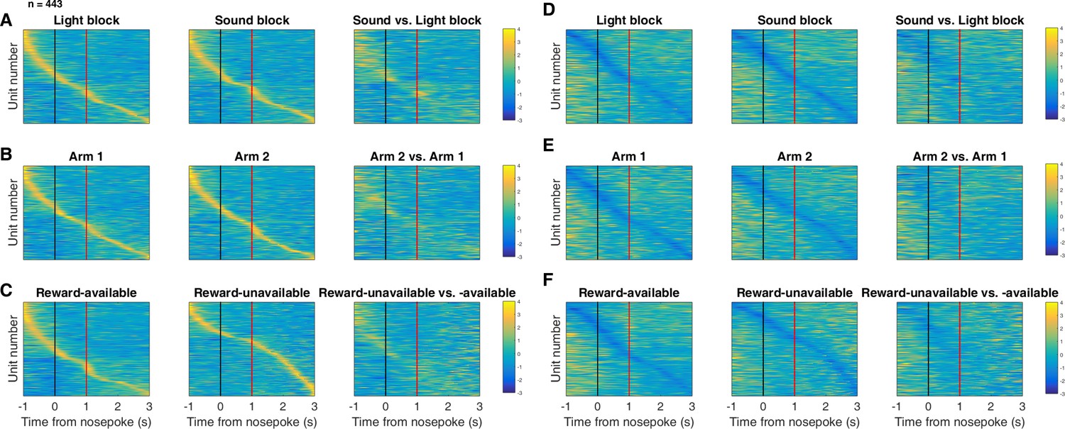
Distribution of NAc firing rates across time surrounding nosepoke for approach trials.
Each panel shows normalized (z-score) firing rates for all recorded NAc units (each row corresponds to one unit) as a function of time (time 0 indicates nosepoke), averaged across all approach trials for a specific cue type, indicated by text labels. (A-C) Heat plots aligned to normalized peak firing rates. (A) left: Heat plot showing smoothed normalized firing activity of all recorded NAc units ordered according to the time of their peak firing rate during the light block. Each row is a unit’s average activity across time to the light block. Black dashed line indicates nosepoke. Red dashed line indicates reward delivery occurring 1 s after nosepoke for reward-available trials. Notice the yellow band across time, indicating all aspects of visualized task space were captured by the peak firing rates of various units. (A) middle: Same units ordered according to the time of the peak firing rate during the sound block. Note that for both blocks, units tile time approximately uniformly with a clear diagonal of elevated firing rates, and a clustering around outcome receipt. (A) right: Unit firing rates taken from the sound block, ordered according to peak firing rate taken from the light block. Note that a weaker but still discernible diagonal persists, indicating partial similarity between firing rates in the two blocks. Colour bar displays relationship between z-score and colour. (B) Same layout as in A, except that the panels now compare two different locations on the track instead of two cue modalities. As for the different cue modalities, NAc units clearly discriminate between locations, but also maintain some similarity across locations, as evident from the visible diagonal in the right panel. Two example locations were used for display purposes; other location pairs showed a similar pattern. (C) Same layout as in A, except that panels now compare correct reward-available and incorrect reward-unavailable trials. The disproportionate coding around outcome receipt for reward-available, but not reward-unavailable trials suggests encoding of reward receipt by NAc units. (D-F) Heat plots aligned to normalized minimum firing rates. (D) Responses during different stimulus blocks as in A, but with units ordered according to the time of their minimum firing rate. (E) Responses during trials on different arms as in B, but with units ordered by their minimum firing rate. (F) Responses during cues signalling different outcomes as in C, but with units ordered by their minimum firing rate. Overall, NAc units coded experience on the task, as opposed to being confined to specific task events only. Units from all sessions and animals were pooled for this analysis.
Figure 8
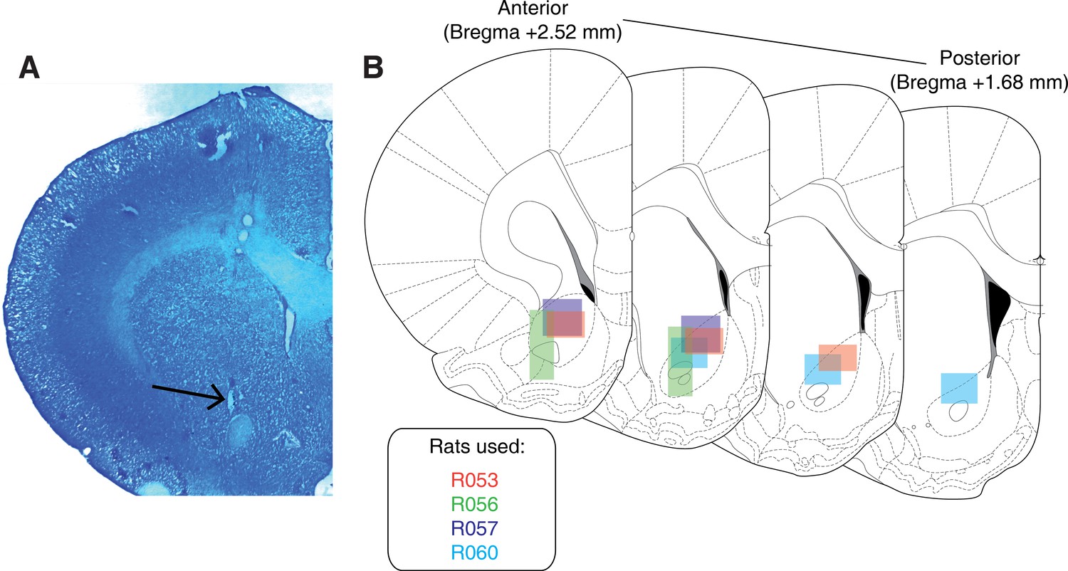
Histological verification of recording sites.
Upon completion of experiments, brains were sectioned and tetrode placement was confirmed. (A) Example section from R060 showing a recording site in the NAc core just dorsal to the anterior commissure (arrow). (B) Schematic showing recording areas for all subjects.
Tables
Table 1
Overview of recorded NAc units and their relationship to task variables at various time epochs.
Percentage is relative to the number of cue-modulated units (n = 133).
| Task parameter | Total | MSN | MSN | FSI | FSI |
|---|---|---|---|---|---|
| All units | 443 | 155 | 216 | 27 | 45 |
| Rat ID | |||||
| R053 | 145 | 51 | 79 | 4 | 11 |
| R056 | 70 | 12 | 13 | 17 | 28 |
| R057 | 136 | 55 | 75 | 3 | 3 |
| R060 | 92 | 37 | 49 | 3 | 3 |
| Analysed units | 344 | 117 | 175 | 18 | 34 |
| Cue modulated units | 133 | 24 | 85 | 6 | 18 |
| GLM aligned to cue-onset | |||||
| Cue identity | 42 (32%) | 9 (38%) | 25 (29%) | 0 (-) | 8 (44%) |
| Cue location | 55 (41%) | 11 (46%) | 33 (39%) | 3 (50%) | 8 (44%) |
| Cue outcome | 26 (20%) | 5 (21%) | 15 (18%) | 1 (17%) | 5 (28%) |
| Approach behaviour | 32 (24%) | 8 (33%) | 19 (22%) | 2 (33%) | 3 (17%) |
| Trial length | 22 (17%) | 5 (21%) | 14 (16%) | 0 (-) | 3 (17%) |
| Trial number | 42 (32%) | 11 (46%) | 20 (24%) | 1 (17%) | 10 (56%) |
| Trial history | 8 (6%) | 1 (4%) | 5 (6%) | 0 (-) | 1 (6%) |
| GLM aligned to nosepoke | |||||
| Cue identity | 28 (21%) | 3 (13%) | 17 (20%) | 2 (33%) | 6 (33%) |
| Cue location | 30 (23%) | 2 (8%) | 21 (25%) | 2 (33%) | 5 (28%) |
| Cue outcome | 23 (17%) | 2 (8%) | 14 (16%) | 1 (17%) | 6 (33%) |
| GLM aligned to outcome | |||||
| Cue identity | 25 (19%) | 4 (17%) | 15 (18%) | 2 (33%) | 4 (22%) |
| Cue location | 31 (23%) | 5 (21%) | 23 (27%) | 0 (-) | 3 (17%) |
| Cue outcome | 34 (26%) | 6 (25%) | 15 (18%) | 4 (67%) | 9 (50%) |
Additional files
-
Transparent reporting form
- https://doi.org/10.7554/eLife.37275.020
Download links
A two-part list of links to download the article, or parts of the article, in various formats.
Downloads (link to download the article as PDF)
Open citations (links to open the citations from this article in various online reference manager services)
Cite this article (links to download the citations from this article in formats compatible with various reference manager tools)
Persistent coding of outcome-predictive cue features in the rat nucleus accumbens
eLife 7:e37275.
https://doi.org/10.7554/eLife.37275


