Humans strategically shift decision bias by flexibly adjusting sensory evidence accumulation
- Max Planck Institute for Human Development, Germany
- University Medical Center Hamburg-Eppendorf, Germany
- University of Amsterdam, The Netherlands
- Vrije Universiteit, The Netherlands
Figures
Figure 1
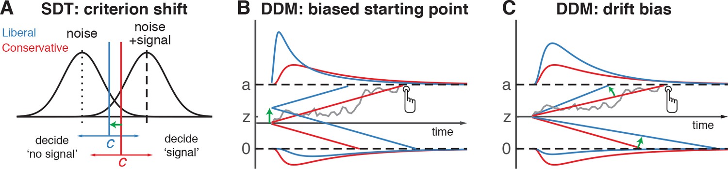
Theoretical accounts of decision bias.
(A) Signal-detection-theoretic account of decision bias. Signal and noise + signal distributions are plotted as a function of the strength of internal sensory evidence. The decision point (or criterion) that determines whether to decide signal presence or absence is plotted as a vertical criterion line c, reflecting the degree of decision bias. c can be shifted left- or rightwards to denote a more liberal or conservative bias, respectively (green arrow indicates a shift toward more liberal). (B, C) Drift diffusion model (DDM) account of decision bias, in which decisions are modelled in terms of a set of parameters that describe a dynamic process of sensory evidence accumulation toward one of two decision bounds. When sensory input is presented, evidence starts to accumulate (drift) over time after initialization at the starting point z. A decision is made when the accumulated evidence either crosses decision boundary a (signal presence) or decision boundary 0 (no signal). After a boundary is reached, the corresponding decision can be either actively reported by a button press (e.g. for signal-present decisions), or remain implicit, without a response (for signal-absent decisions). The DDM can capture decision bias through a shift of the starting point of the evidence accumulation process (panel B) or through a shift in bias in the rate of evidence accumulation toward the different choices (panel C). These mechanisms are dissociable through their differential effect on the shape of the reaction time (RT) distributions, as indicated by the curves above and below the graphs for target-present and target-absent decisions, respectively. Panels B. and C. are modified and reproduced with permission from Urai et al., 2018 (Figure 1, published under a CC BY 4.0 license).
Figure 2 with 3 supplements

Strategic decision bias shift toward liberal biases evidence accumulation.
(A) Schematic of the visual stimulus and task design. Participants viewed a continuous stream of full-screen diagonally, horizontally and vertically oriented textures at a presentation rate of 40 ms (25 Hz). After random inter-trial intervals, a fixed-order sequence was presented embedded in the stream. The fifth texture in each sequence either consisted of a single diagonal orientation (target absent), or contained an orthogonal orientation-defined square (either 45° or 135° orientation). Participants decided whether they had just seen a target, reporting detected targets by button press. Liberal and conservative conditions were administered in alternating nine-min blocks by penalizing either misses or false alarms, respectively, using aversive tones and monetary deductions. Depicted square and fixation dot sizes are not to scale. (B) Average detection rates (hits and false alarms) during both conditions. Miss rate is equal to 1 – hit rate since both are computed on stimulus present trials, and correct-rejection rate is equal to 1 – false alarm rate since both are computed on stimulus absent trials, together yielding the four SDT stimulus-response categories. (C) SDT parameters for sensitivity and criterion. (D) Schematic and simplified equation of drift diffusion model accounting for reaction time distributions for actively reported target-present and implicit target-absent decisions. Decision bias in this model can be implemented by either shifting the starting point of the evidence accumulation process (Z), or by adding an evidence-independent constant (‘drift bias’, db) to the drift rate. See text and Figure 1 for details. Notation: dy, change in decision variable y per unit time dt; v·dt, mean drift (multiplied with one for signal + noise (target) trials, and −1 for noise-only (nontarget) trials); db·dt, drift bias; and cdW, Gaussian white noise (mean = 0, variance = c2·dt). (E) Difference in Bayesian Information Criterion (BIC) goodness of fit estimates for the drift bias and the starting point models. A lower delta BIC value indicates a better fit, showing superiority of the drift bias model to account for the observed results. (F) Estimated model parameters for drift rate and drift bias in the drift bias model. Error bars, SEM across 16 participants. ***p<0.001; n.s., not significant. Panel D. is modified and reproduced with permission from de Gee et al. (2017) (Figure 4A, published under a CC BY 4.0 license).
-
Figure 2—source data 1
This csv table contains the data for Figure 2 panels B, C, E and F.
- https://doi.org/10.7554/eLife.37321.008
Figure 2—figure supplement 1
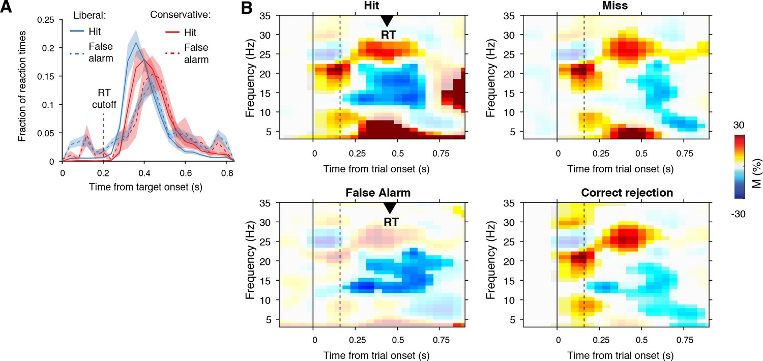
Behavioral and neurophysiological evidence that participants were sensitive to the implicit task structure.
(A) Participant-average RT distributions for hits and false alarms in both conditions. The presence of similar RT distributions for false alarms and hits indicates that participants were sensitive to trial onset despite the fact that trial onsets were only implicitly signaled. Error bars, SEM. (B) Time-frequency representations of low-frequency EEG power modulations with respect to the pre-stimulus period (–0.4–0 s), pooled across the two conditions. Significant low-frequency modulation occurred even for nontarget trials without overt response (correct rejections), indicating that participants detected the onset of a trial even when neither a target was presented nor a response was given. Saturated colors indicate clusters of significant modulation, cluster threshold p<0.05, two-sided permutation test across participants, cluster- corrected; N = 15). Solid and dotted vertical lines respectively indicate the onset of the trial and the target stimulus. M, power modulation.
Figure 2—figure supplement 2
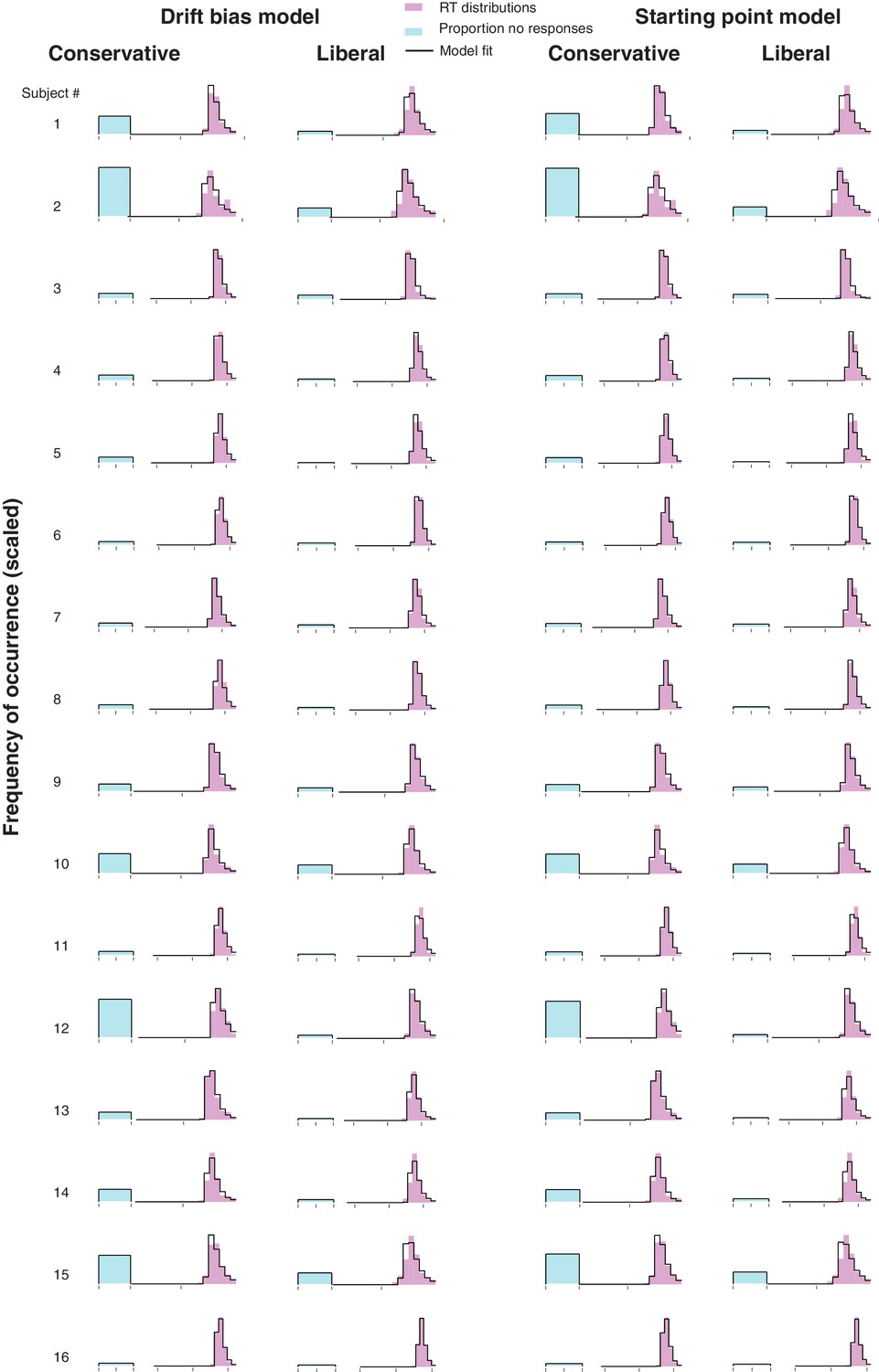
Single-participant drift diffusion model fits for the drift bias and starting point models for both conditions.
Rows, single participant RT distributions and drift diffusion model fits for the two models for both conditions.
Figure 2—figure supplement 3
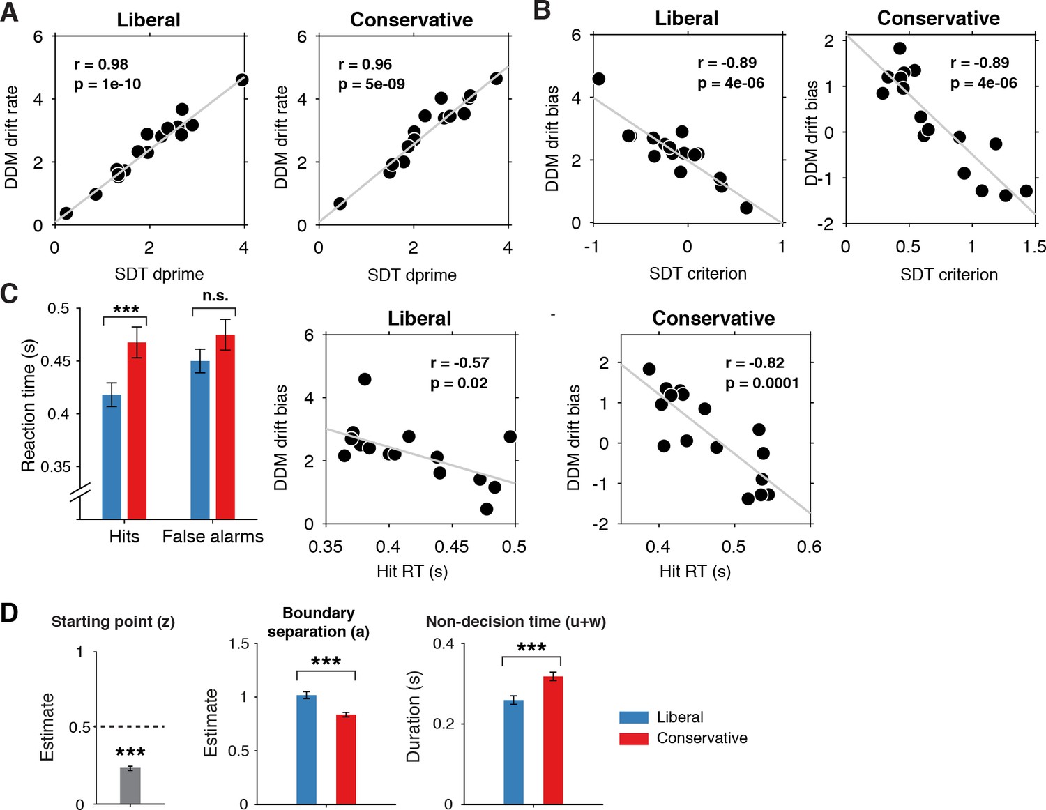
Signal-detection-theoretic (SDT) behavioral measures during both conditions correspond closely to drift diffusion modeling (DDM) parameters.
(A) Across-participant Pearson correlation between d’ and drift rate for the two conditions. Each dot represents a participant. (B) As A. but for correlation between criterion and DDM drift bias. The correlation is negative due to a lower criterion reflecting a stronger liberal bias. (C) Left panel, mean reaction times (RT) for hits and false alarms for the two conditions. Middle and right panels, As A. but for correlation between RT for hits and drift bias. (D) Parameter estimates in the drift bias DDM not related to evidence accumulation (drift rate). ***p<0.001; n.s., not significant.
Figure 3
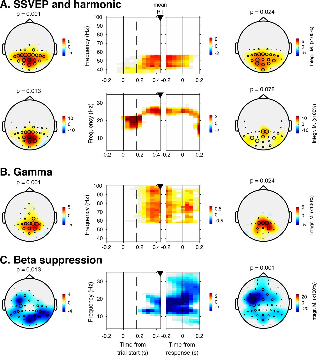
EEG spectral power modulations related to stimulus processing and motor response.
Each panel row depicts a three-dimensional (electrodes-by-time-by-frequency) cluster of power modulation, time-locked both to trial onset (left two panels) and button press (right two panels). Power modulation outside of the significant clusters is masked out. Modulation was computed as the percent signal change from the condition-specific pre-stimulus period (–0.4 to 0 s) and averaged across conditions. Topographical scalp maps show the spatial extent of clusters by integrating modulation over time-frequency bins. Time-frequency representations (TFRs) show modulation integrated over electrodes indicated by black circles in the scalp maps. Circle sizes indicate electrode weight in terms of proportion of time-frequency bins contributing to the TFR. P-values above scalp maps indicate multiple comparison-corrected cluster significance using a permutation test across participants (two-sided, N = 14). Solid vertical lines indicate the time of trial onset (left) or button press (right), dotted vertical lines indicate time of (non)target onset. Integr. M., integrated power modulation. SSVEP, steady state visual evoked potential. (A) (Top) 42–58 Hz (SSVEP harmonic) cluster. (A) (Bottom). Posterior 23–27 Hz (SSVEP) cluster. (B) Posterior 59–100 Hz (gamma) cluster. The clusters in A (Top) and B were part of one large cluster (hence the same p-value), and were split based on the sharp modulation increase precisely in the 42–58 Hz range. (C) 12–35 Hz (beta) suppression cluster located more posteriorly aligned to trial onset, and more left-centrally when aligned to button press.
Figure 4

Experimental task manipulations affect the time course of stimulus- and motor-related EEG signals, but not its starting point.
Raw power throughout the baseline period and time courses of power modulation time-locked to trial start and button press. (A) Relevant electrode clusters and frequency ranges (from Figure 3): Posterior SSVEP, Posterior gamma and Left-hemispheric beta (LHB). (B) The time course of raw power in a wide interval around the stimulus –0.8 to 0.8 s ms for these clusters. (C) Stimulus locked and response locked percent signal change from baseline (baseline period: –0.4 to 0 s). Error bars, SEM. Black horizontal bar indicates significant difference between conditions, cluster-corrected for multiple comparison (p<0.05, two sided). SSVEP, steady state visual evoked potential; LHB, left hemispheric beta; ERP, event-related potential; SCD, scalp current density.
Figure 5
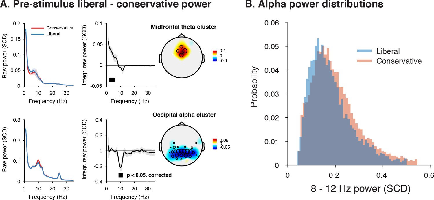
Adopting a liberal decision bias is reflected in increased midfrontal theta and suppressed pre-stimulus alpha power.
(A) Significant clusters of power modulation between liberal and conservative in a pre-stimulus window between −1 and 0 s before trial onset. When performing a cluster-based permutation test over all frequencies (1–35 Hz) and electrodes, two significant clusters emerged: theta (2–6 Hz, top), and alpha (8–12 Hz, bottom). Left panels: raw power spectra of pre-stimulus neural activity for conservative and liberal separately in the significant clusters (for illustration purposes), Middle panels: Liberal – conservative raw power spectrum. Black horizontal bar indicates statistically significant frequency range (p<0.05, cluster-corrected for multiple comparisons, two-sided). Right panels: Corresponding liberal – conservative scalp topographic maps of the pre-stimulus raw power difference between conditions for EEG theta power (2–6 Hz) and alpha power (8–12 Hz). Plotting conventions as in Figure 3. Error bars, SEM across participants (N = 15). (B) Probability density distributions of single trial alpha power values for both conditions, averaged across participants.
Figure 6 with 1 supplement

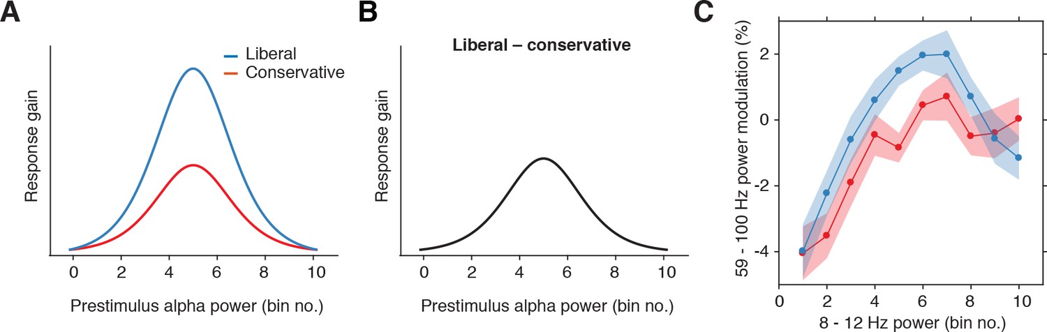
Pre-stimulus alpha power is linked to cortical gamma responses.
(A) Theoretical response gain model describing the transformation of stimulus-induced and endogenous input activity (denoted by Sx and SN respectively) to the total output activity (denoted by O(Sx +SN)) in visual cortex by a sigmoidal function. Different operational alpha ranges are associated with input-output functions with different slopes due to corresponding changes in the total output. (B) Alpha-linked output responses (solid lines) are formalized as the first derivative (slope) of the sigmoidal functions (dotted lines), resulting in inverted-U (Gaussian) shaped relationships between alpha and gamma, involving stronger response gain in the liberal than in the conservative condition. (C) Corresponding empirical data showing gamma modulation (same percent signal change units as in Figure 3) as a function of alpha bin. The location on the x-axis of each alpha bin was taken as the median alpha of the trials assigned to each bin and averaged across subjects. (D-F) Model prediction tests. (D) Raw pre-stimulus alpha power for both conditions, averaged across subjects. (E) Post-stimulus gamma power modulation for both conditions averaged across the two middle alpha bins (5 and 6) in panel C. (F) Liberal – conservative difference between the response gain curves shown in panel C, centered on alpha bin. Error bars, within-subject SEM across participants (N = 14).
-
Figure 6—source data 1
SPSS .sav file containing the data used in panels C, E, and F.
- https://doi.org/10.7554/eLife.37321.014
Figure 6—figure supplement 1
Gain model predictions and corresponding empirical data plotted as a function of pre-stimulus alpha bin number.
(A) Model predictions for both conditions. The gain curve for the liberal condition is steeper than for the conservative condition. Binning trials based on alpha within each condition directly maps the peaks of the gain curves onto each other. (B) Model prediction for liberal – conservative as a function of alpha bin number. The difference gain curve between the two conditions is again an inverted-U shaped function. (C) Corresponding empirical data. The plot is identical to Figure 5C, except that the bin number is plotted instead of the actual alpha power for each condition.
Figure 7 with 1 supplement
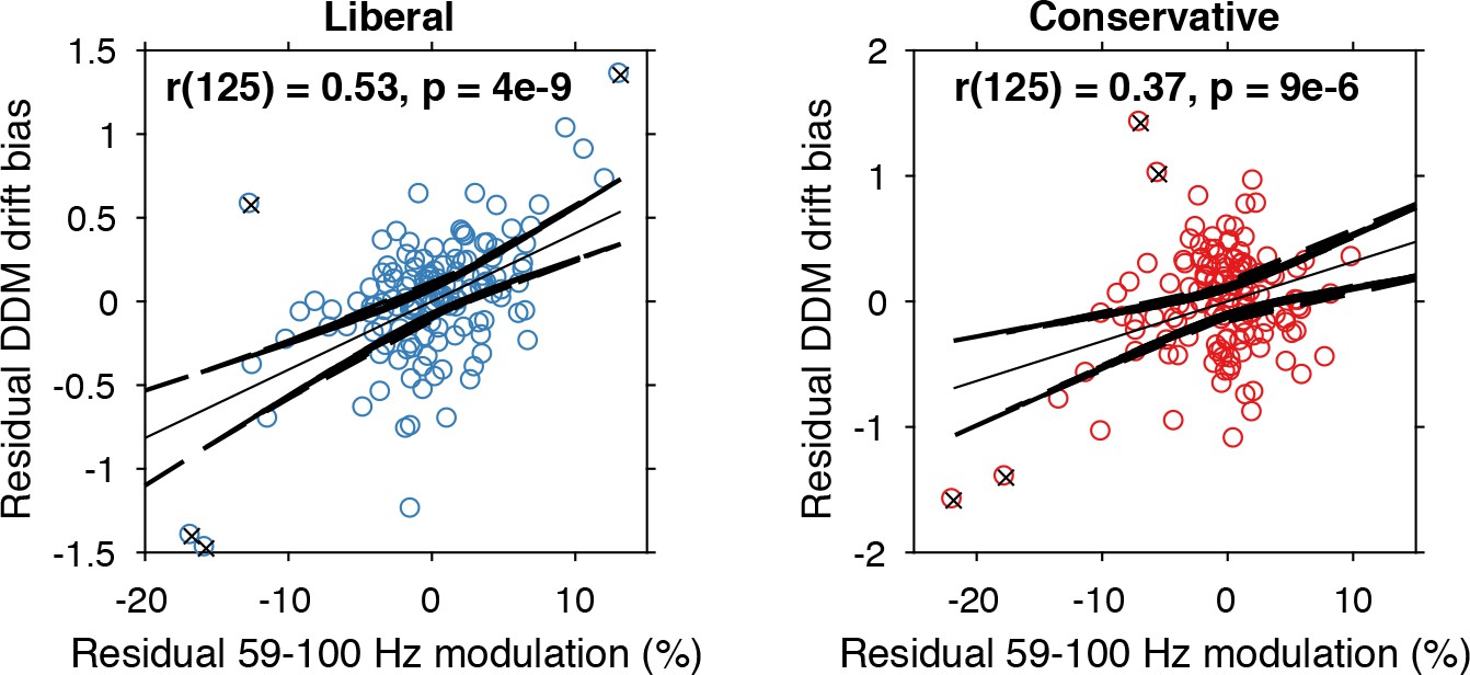
Alpha-binned gamma modulation correlates with evidence accumulation bias.
Repeated measures correlation between gamma modulation and drift bias for the two conditions. Each circle represents a participant’s gamma modulation within one alpha bin. Drift bias and gamma modulation scalars were residualized by removing the average within each participant and condition, thereby removing the specific range in which the participants values operated. Crosses indicate data points that were most influential for the correlation, identified using Cook’s distance. Correlations remained qualitatively unchanged when these data points were excluded (liberal, r(120) = 0.46, p=8e-07; conservative, r(121) = 0.27, p=0.0009) Error bars, 95% confidence intervals after averaging across participants.
-
Figure 7—source data 1
MATLAB .mat file containing the data used.
- https://doi.org/10.7554/eLife.37321.017
Figure 7—figure supplement 1
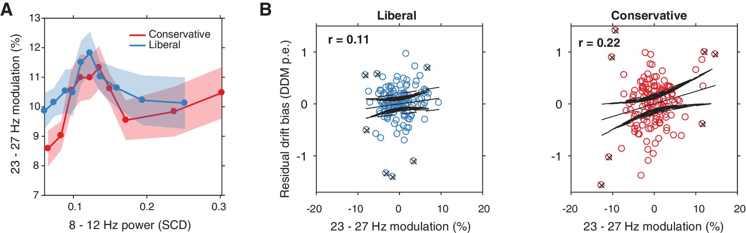
Alpha-binned post-stimulus SSVEP modulation.
(A) Inverted-U shaped relationship between alpha and SSVEP modulation, computed as the percent signal change 23–27 Hz power modulation with respect to the pre-stimulus baseline. (B) Correlations between SSVEP modulation and drift bias for both conditions. These non-significant correlations are overall weaker than for gamma (see Figure 6).
Figure 8
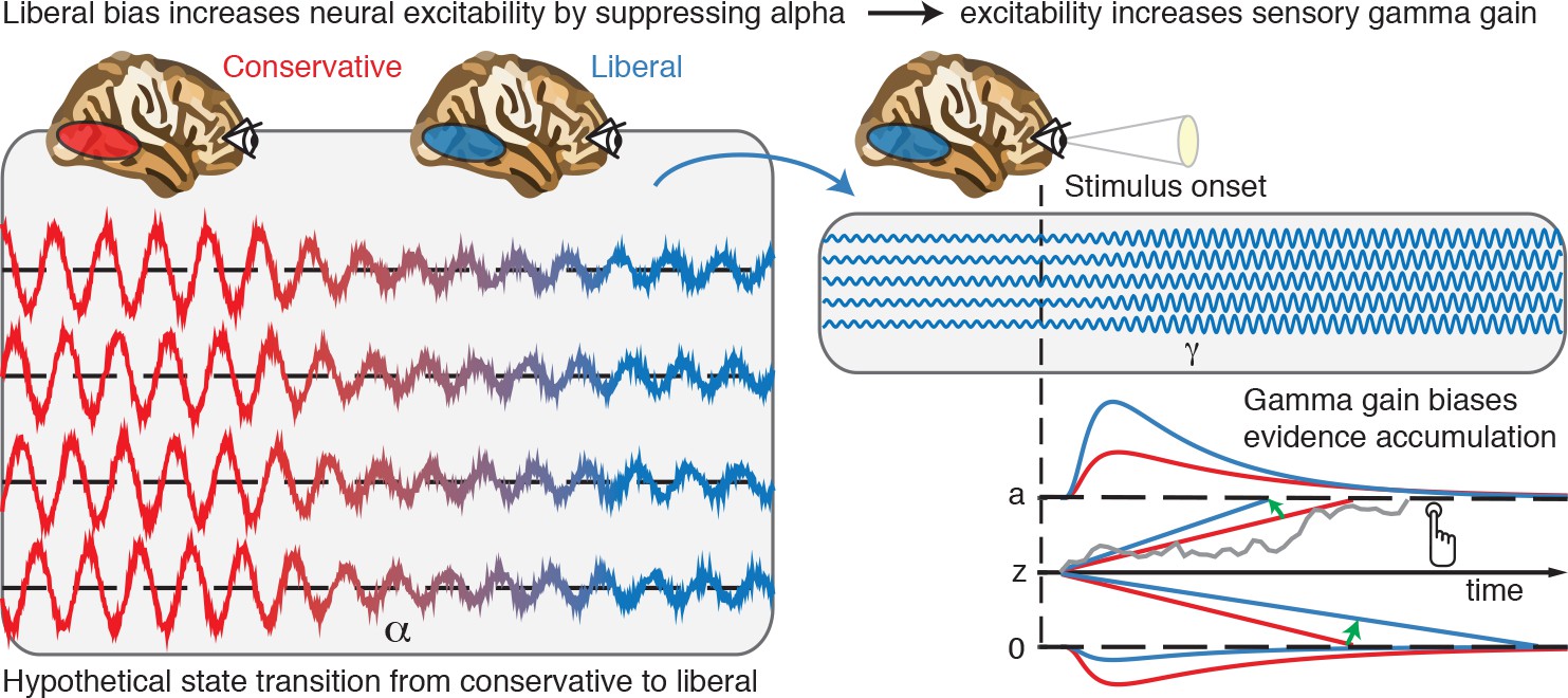
Illustrative graphical depiction of the excitability state transition from conservative to liberal, and subsequent biased evidence accumulation under a liberal bias.
The left panel shows the transition from a conservative to a liberal condition block. The experimental induction of a liberal decision bias causes alpha suppression in visual cortex, which increases neural excitability. The right top panel shows increased gamma gain for incoming sensory evidence under conditions of high excitability. The right bottom panel shows how increased gamma-gain causes a bias in the drift rate, resulting in more ‘target present’ responses than in the conservative state.
Author response image 1
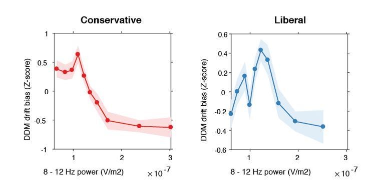
Inverse-U shaped relationship between pre-stimulus alpha power and drift bias.
DDM drift bias parameter estimates were Z-scored within each condition to remove the large inter-individual differences in average drift bias within each condition and focus on the shape of the relationship between alpha and drift bias. Therefore, the difference in average drift bias between conditions (see Figure 2F) is not reflected in these figures.
Tables
Key resources table
| Reagent type (species) or resource | Designation | Source or reference | Identifiers | Additional information |
|---|---|---|---|---|
| Biological sample (Humans) | Participants | This paper | See Participants section in Materials and methods | |
| Software, algorithm | MATLAB | Mathworks | MATLAB_R2016b, RRID:SCR_001622 | |
| Software, algorithm | Presentation | NeuroBS | Presentation_v9.9, RRID:SCR_002521 | |
| Software, algorithm | Custom analysis code | Kloosterman, 2018 | https://github.com/nkloost1/critEEG | |
| Other | EEG data experimental task | Kloosterman et al., 2018 | https://doi.org/10.6084/m9.figshare.6142940 |
Additional files
-
Transparent reporting form
- https://doi.org/10.7554/eLife.37321.019
Download links
A two-part list of links to download the article, or parts of the article, in various formats.
Downloads (link to download the article as PDF)
Open citations (links to open the citations from this article in various online reference manager services)
Cite this article (links to download the citations from this article in formats compatible with various reference manager tools)
Humans strategically shift decision bias by flexibly adjusting sensory evidence accumulation
eLife 8:e37321.
https://doi.org/10.7554/eLife.37321


