Elementary sensory-motor transformations underlying olfactory navigation in walking fruit-flies
- New York University Langone Medical Center, United States
- University of Colorado Boulder, United States
- Weill Cornell Medical College, United States
Figures
Figure 1 with 3 supplements
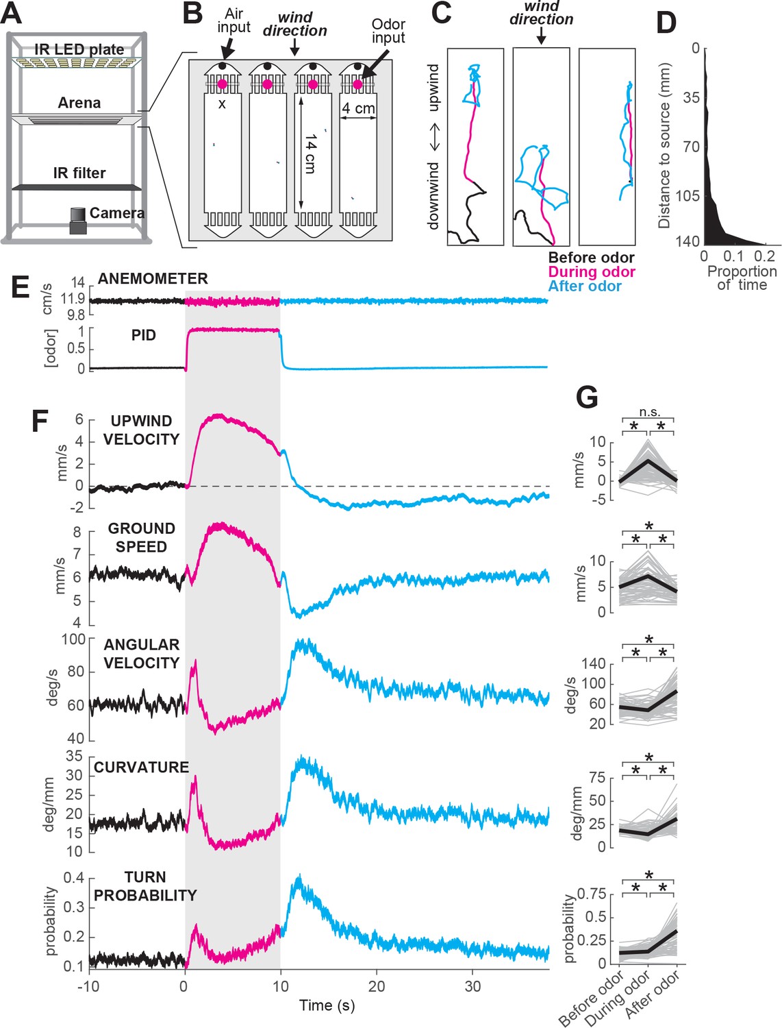
ON and OFF responses to an attractive odor pulse.
(A) Schematic of the behavioral apparatus (side view) showing illumination and imaging camera. (B) Schematic of the behavioral arena (top view) showing four behavior chambers and spaces to direct air and odor through the apparatus. Dots mark air and odor inputs. Black cross: site of wind and odor measurements in E. (C) Example trajectories of three different flies before (black), during (magenta) and after (cyan) a 10 s odor pulse showing upwind runs during odor and search after odor offset. (D) Distribution of fly positions on trials with wind and no odor; flies prefer the downwind end of the arena. (E) Average time courses of wind (top; anemometer measurement; n = 10) and odor (bottom; PID measurement normalized to maximal concentration; n = 10) during 10 s odor trials. Measurements were made using 10% ethanol at the arena position shown in B. (F) Calculated parameters of fly movement averaged across flies (meanSEM; n = 75 flies, 1306 trials; see Materials and methods). Traces are color coded as in C. Gray-shaded area: odor stimulation period (ACV 10%). All traces warped to estimated time of odor encounter and loss prior to averaging. Small deflections in ground speed near the time of odor onset and offset represent a brief stop response to the click of the odor valves (see Figure 3—figure supplement 1). (G) Average values of motor parameters in F for each fly for periods before (−30 to 0 s), during (2 to 3 s) and after (11 to 13 s) the odor. Gray lines: data from individual flies. Black lines: group average. Horizontal lines with asterisk: Statistically significant changes in a Wilcoxon signed rank paired test after correction for multiple comparisons using the Bonferroni method (see Materials and methods for p values). n.s.: not significant.
Figure 1—figure supplement 1
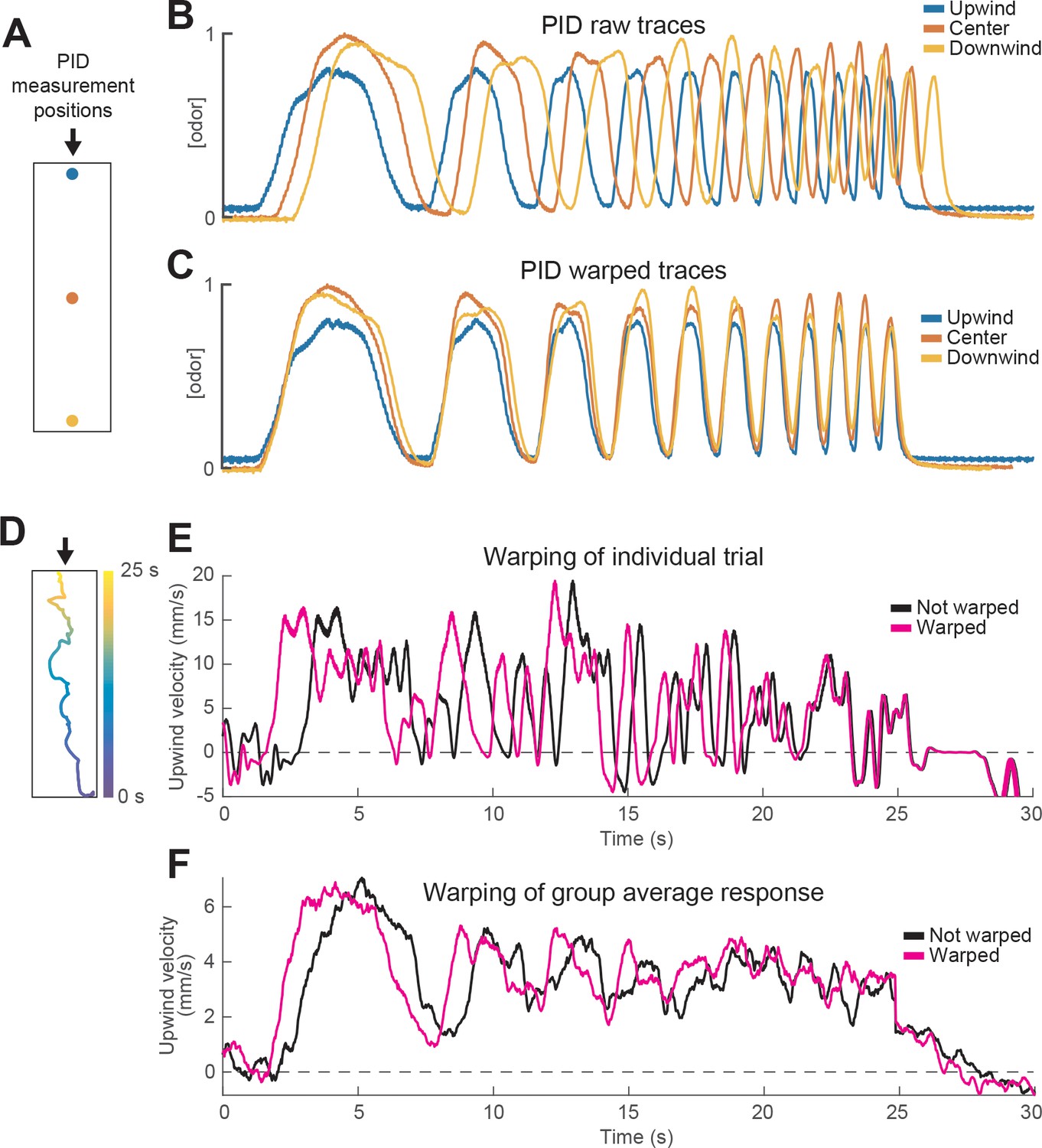
Warping method corrects for differences in odor encounter timing as a function of position within the arena.
(A) Schematic of the behavioral arena marking different points at which we measured the odor waveform by PID. Arrow signals wind direction. (B) PID measurements of an upward frequency sweep stimulus recorded at the three points in A using 10% ethanol. Note the delay between the stimulus measured at the source (blue) and the one measured at the bottom of the arena (yellow). (C) Same PID traces as in B after warping traces measured downwind of the source (red and yellow). Note the overlap between the three traces in each phase of the stimulus. (D) Trajectory of a fly in a single trial while experiencing the stimulus depicted in C. Time in the stimulus (0–25 s) is color coded, showing that the fly moved from the bottom of the arena to the top during the stimulus. (E) Upwind velocity of the fly in the example trial shown in D. Black trace represents raw upwind velocity. Magenta trace shows data after warping. Note that warping reduces the apparent latency of the first behavioral response, and that the difference between the traces decreases as the fly approaches the odor source F) Same as E, but traces represent the mean upwind velocity of a group of flies in response to the same stimulus (n = 31 flies, 346 trials; data in Figure 3E). Note that warping improves the phasic structure in the data.
Figure 1—figure supplement 2

Variability between individuals in responses to an odor pulse.
(A) Example trajectories from two different flies (left and right groups), from non-consecutive trials, in response to a 10 s odor pulse. Left hand fly: weak searcher, right-hand fly: strong searcher. (B) Mean upwind velocity during odor (2 to 3 s) and turn probability after odor (11 to 13 s) for each fly (n = 75 flies; data in Figure 1). Each point represents the average of a single fly (meanSEM). Dashed lines: group average values for ON and OFF responses. Green and blue dots: weak- and strong-searching flies featured in panels A and C. Data from these flies is used in Figure 5J and K. (C) Average upwind velocity and turn probability of weak- and strong-searching flies in B, and of the whole group (gray traces; n = 75 flies, 1306 trials), in response to a 10 s odor pulse. (D) Flies exhibit characteristic search strengths. Left plot: upwind velocity for each fly on half of trials versus upwind velocity in remaining trials (n = 75 flies; trials for each half were randomly selected). Each point represents mean upwind velocity 2–3 s after odor onset for each fly in Figure 1. Middle plot: same analysis performed on trials where fly identity was scrambled. Right plot: Quantification of correlations for upwind velocity during odor, ground speed before odor, and turn probability at offset. Each bar shows the correlation coefficient (meanSTD) from 10 repetitions of the corresponding correlation, either with fly identity preserved (filled bars), or scrambling the data (blank bars). Ground speed (GS) was taken from −30 to 0 s before odor. Upwind velocity (UV) was taken from 2 to 3 s during odor. Turn probability (TP) was taken from 1 to 3 s after odor. (E) Trial-by-trial correlation coefficients between movement parameters (computed for each fly, then averaged across flies; n = 75 flies). ON parameters are correlated with each other, as are OFF parameters, but ON and OFF are not correlated with each other. This suggests that ON and OFF responses are separately regulated on a trial by trial basis. : Mean ground speed from 2 to 3 s during odor. : Mean upwind velocity from 2 to 3 s during odor. : Mean angular velocity from 1 to 3 s after odor. : Mean curvature from 1 to 3 s after odor. : Mean turn probability from 1 to 3 s after odor. (F) Mean upwind velocity from 2 to 3 s during odor for each trial of every fly in Figure 1 in which the stimulus was a 10 s odor pulse, represented in chronological order along the X axis. Gray lines: data from individual flies. Black traces: Area between SEM errors.
Figure 1—figure supplement 3
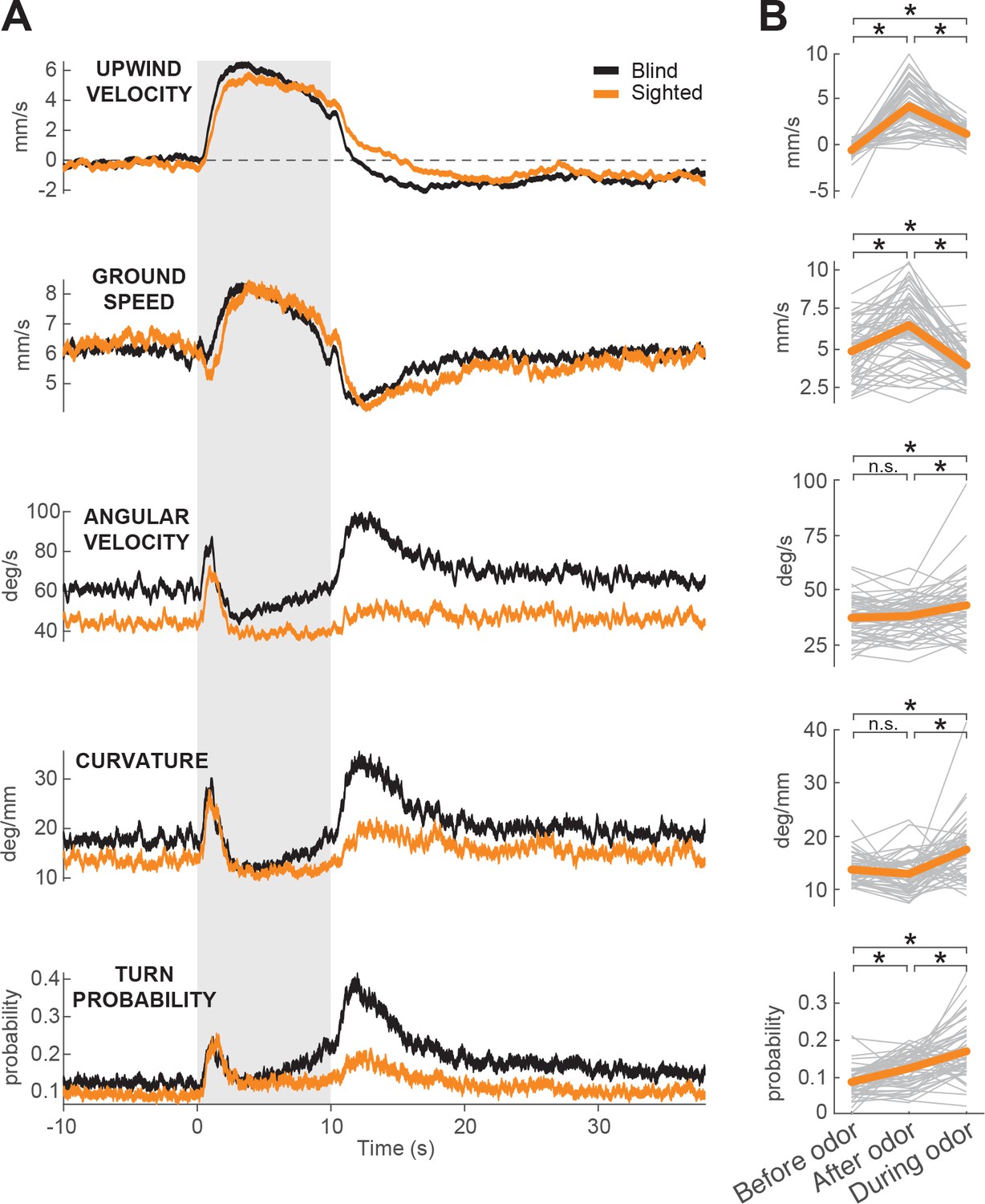
Sighted flies show ON and OFF responses to odor.
(A) Calculated parameters of fly movement averaged across flies (meanSEM). Black traces represent responses of blind flies w1118 5905 norpA (Kennedy, 1940) (same data as in Figure 1F; n = 75 flies, 1306 trials). Orange traces are responses of sighted flies w1118 5905 (n = 56 flies, 1155 trials; see Materials and methods). Gray-shaded area: odor stimulation period (ACV 10%). All traces warped to estimated time of odor encounter and loss prior to averaging. Small deflections in ground speed near the time of odor onset and offset represent a brief stop response to the click of the odor valves (see Figure 3—figure supplement 1E). (B) Average values of motor parameters in A for each fly for periods before (−30 to 0 s), during (2 to 3 s) and after (11 to 13 s) the odor. Gray lines: data from individual flies. Orange thicker lines: group average. Horizontal lines with asterisk: Statistically significant changes in a Wilcoxon signed rank paired test after correction for multiple comparisons using the Bonferroni method (see Materials and methods for p values). n.s.: not significant.
Figure 2
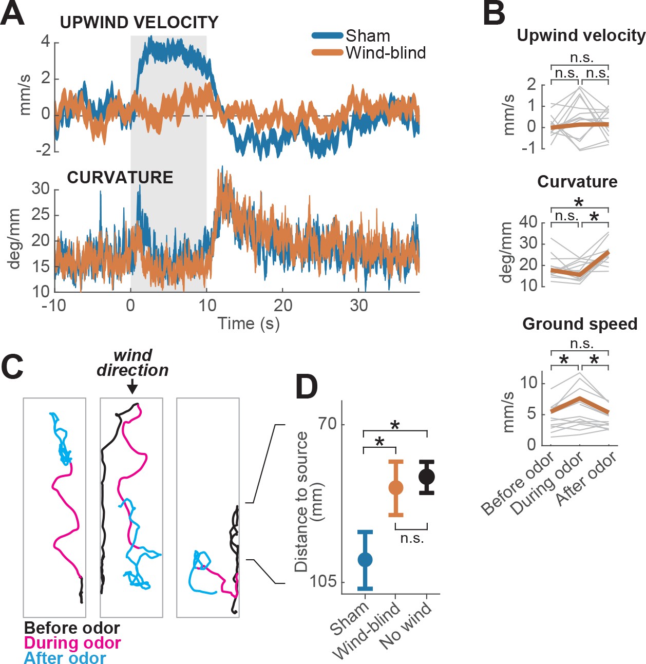
Multimodal and unimodal contributions to olfactory behavior.
(A) Stabilization of the antennae abolishes odor-evoked changes in upwind velocity but not curvature. Traces show meanSEM for wind-blind (n = 13 flies, 240 trials) and sham-treated flies (n = 15 flies, 217 trials; see Materials and methods) (B) Mean values of upwind velocity, curvature and ground speed in wind-blind flies during periods before, during, and after the odor pulse (time windows as in Figure 1G). Gray lines: data from individual wind-blind flies. Orange lines: group average. Horizontal lines with asterisk: statistically significant changes in a Wilcoxon signed rank paired test after correction for multiple comparisons using the Bonferroni method (see Materials and methods for p values). n.s.: not significant. (C) Example trajectories of three different wind-blind flies before (black), during (magenta) and after (cyan) the odor pulse. Note different orientations relative to wind during the odor. (D) Antenna stabilization decreases preference for the downwind end of the arena on trials with wind and no odor. Blue: average (SEM) arena position of sham-treated flies on trials with wind and no odor. Orange: average position of wind-blind flies in the same stimulus condition. Black: Average position of intact (not-treated) flies in the absence of both odor and wind (n = 23 flies, 1004 trials). The average arena position of wind-blind flies did not differ significantly from that of no-wind flies (p=0.93). Sham-treated flies spent significantly more time downwind than wind-blind (p=0.04) or intact flies in the absence of wind (p=0.0027). Horizontal lines with asterisk: statistically significant changes in a Wilcoxon rank sum test (alpha = 0.05). n.s.: non-significant. Black lines between C and D provided for reference of dimensions in D.
Figure 3 with 1 supplement
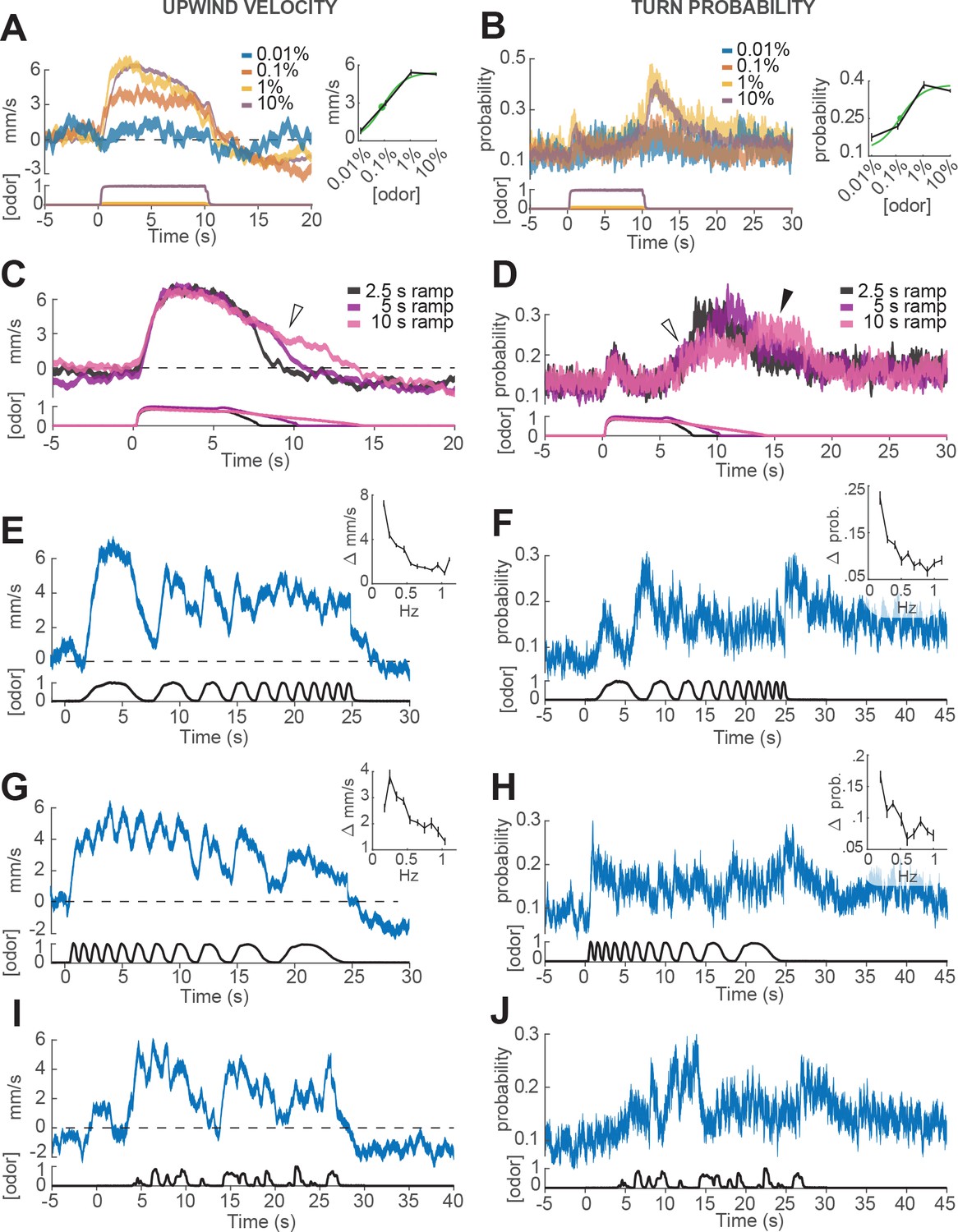
Responses of walking flies to dynamic odor stimuli.
(A) Upwind velocity (left, top traces; averageSEM) of different groups of flies responding to a 10 s pulse of ACV at dilutions of 0.01% (n = 13 flies, 147 trials), 0.1% (n = 19 flies, 304 trials), 1% (n = 18 flies, 302 trials) and 10% (n = 75 flies, 1306 trials). Left-bottom traces show PID measurements using ethanol (max concentration 10%), normalized to maximal amplitude. Right inset: mean upwind velocity during odor (2 to 3 s) as a function of odor concentration (black; meanSEM), and fitted Hill function (green; green dot: =0.072%). (B) Turn probability calculated from the same data. Right inset black traces: mean turn probability after odor (11 to 13 s). =0.127% for fitted Hill function (green). (C) Upwind velocity (averageSEM) in response to stimuli with off-ramps of 2.5 (n = 38 flies, 528 trials), 5 (n = 38 flies, 567 trials) and 10 (n = 35 flies, 557 trials) seconds duration. Bottom traces: PID signals of the same stimuli using ethanol. (D) Same as C, showing turn probability from the same data sets. White arrows in C and D show elevated upwind velocity and turn probability that co-occur during a slow off-ramp. Black arrow in D: peak turn probability response at the foot of the off-ramp. (E) Upwind velocity (meanSEM; n = 31 flies, 346 trials) in response to an ascending frequency sweep stimulus. Bottom trace: PID signal of the stimulus, measured using ethanol. Right inset: average (SEM) modulation of upwind velocity as a function of frequency in each stimulus cycle (see Materials and methods). (F) Same as E for turn probability calculated from the same data. Right inset: modulation of turn probability as a function of frequency. (G) Equivalent to E, showing responses to a descending frequency sweep (n = 33 flies, 345 trials). In the inset, the first high-frequency cycle was left out of the analysis. (H) Same as G for turn probability calculated from the same data. (I) Equivalent to G, showing responses to a simulated ‘plume walk’ (n = 30 flies, 393 trials). (J) Same as I for turn probability calculated from the same data.
Figure 3—figure supplement 1
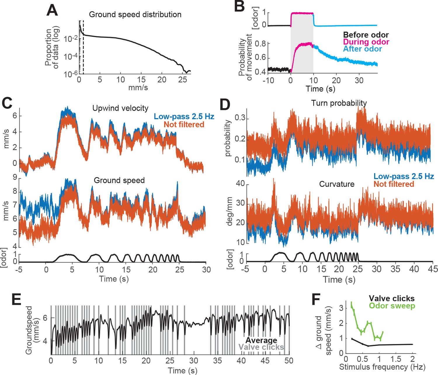
Data processing methods.
(A–C) Segmentation of data into moving and non-moving epochs for analysis. (A) Distribution of ground speed values for all flies during trials with a 10 s odor pulse (n = 75 flies, 1306 trials; data from Figure 1). Y axis on a logarithmic scale. Note large peak close to 0 mm/s corresponding to non-moving epochs. (B) Probability of moving at greater than 1 mm/s increases during odor and remains elevated for tens of seconds after odor offset. PID measurement (top trace) and probability of movement (bottom trace) during a 10 s odor pulse (meanSEM; n = 75 flies, 1306 trials; data from Figure 1). Thus, if non-moving periods are not omitted from computation of movement parameters such as ground speed and angular velocity, the means of these parameters are heavily influenced by the fraction of non-moving flies (i.e. the number of zeros) in each epoch. (C–D) Effects of low-pass filtering on estimates of behavioral responses to fluctuating stimuli. (C) Upwind velocity (top) and ground speed (middle) of flies in response to an ascending frequency sweep stimulus (meanSEM; n = 31 flies, 346 trials; data from Figure 3E). Blue traces: data as it was used in Figure 3. Red traces: data processed exactly as the blue traces, except we omitted the low-pass filtering at 2.5 Hz. Note that the difference between the two sets is small and mostly shows as increased high-frequency noise in the periods before the stimulus. Bottom black trace: stimulus. (D) Same as C, showing turn probability (top) and curvature (middle) in response to the same stimulus. (E–F) Reliable modulation of behavior at high frequencies can be observed in response to valve clicks. (E) Mean ground speed (n = 31 flies, 248 trials) in response to a random train of valve clicks with a 50% probability of occurrence. Vertical gray lines: time at which the odor valves opened or closed, producing a click sound and slight vibration. Note that flies slowed their ground speed after every click. (F) Modulation of ground speed during random valve clicks (black trace; meanSEM (absolute values); n = 31 flies, 248 trials; data in E) and during every cycle of an ascending frequency sweep stimulus (green trace; meanSEM; n = 31 flies, 346 trials; data and analysis in Figure 3E, inset). Frequency of valve clicks ranged from 0.18 to 2 Hz and was calculated as one over the inter-click interval (responses to the first click were ignored).
Figure 4
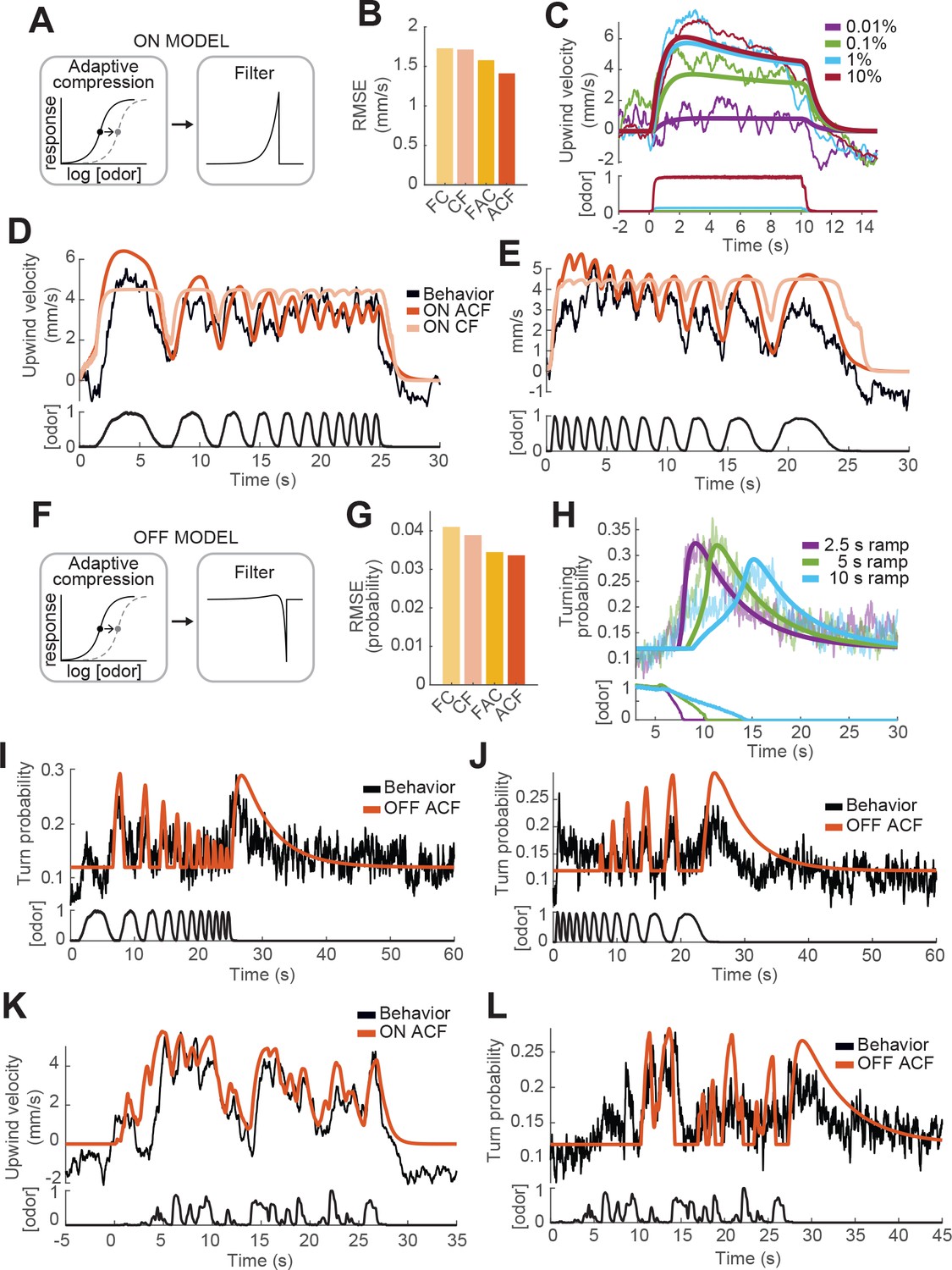
Computational modeling of ON and OFF response functions.
(A) ON model schematic featuring adaptive compression followed by linear filtering. (B) Root mean squared error between predictions of four ON models and behavioral data. FC: filter then compress; CF: compress then filter; FAC: filter then adaptive compression; ACF: adaptive compression then filtering. (C) Upwind velocity of real flies (top thiner traces; average; same data in Figure 3A) and predictions of the ACF ON model (top thicker traces) to square pulses of ACV at different concentrations. Bottom traces: stimuli, normalized to maximal amplitude. Note that adaptation appears only at higher concentrations and that responses saturate between 1% and 10% ACV. (D) Upwind velocity of real flies (top black trace; average; same data in Figure 3E), and predictions of ACF (red) and CF (pink) ON models to an ascending frequency sweep. Bottom trace: stimulus. Note that the model without adaptation (CF) exhibits saturation not seen in the data. (E) Same as D for a descending frequency sweep stimulus (same data in Figure 3G). (F) OFF model schematic featuring adaptive compression followed by differential filtering. (G) Root mean squared error between predictions of four OFF models and behavioral data. (H) Turn probability of real flies (top thiner traces; average; same data in Figure 3D) and predictions of the ACF OFF model (top thicker traces) to odor ramps of different durations. Bottom traces: stimuli. (I) Turn probability (top black trace; average; same data in Figure 3F), and predictions of ACF OFF model (top red trace) to an ascending frequency sweep. Bottom trace: stimulus. (J) Same as I for a descending frequency sweep stimulus (same data in Figure 3H). (K) Upwind velocity (top black trace; average; same data in Figure 3I), and predictions of ACF ON model to the ‘plume walk’ stimulus (see Results). Bottom trace: stimulus. RMSE = 1.355. (L) Same as K for the same stimulus, showing turning probability of real flies (top black trace; average; same data in Figure 3J) and predictions of the ACF OFF model (top red trace). Bottom trace: stimulus. RMSE = 0.038. Plume walk responses were not used to fit the models.
Figure 5
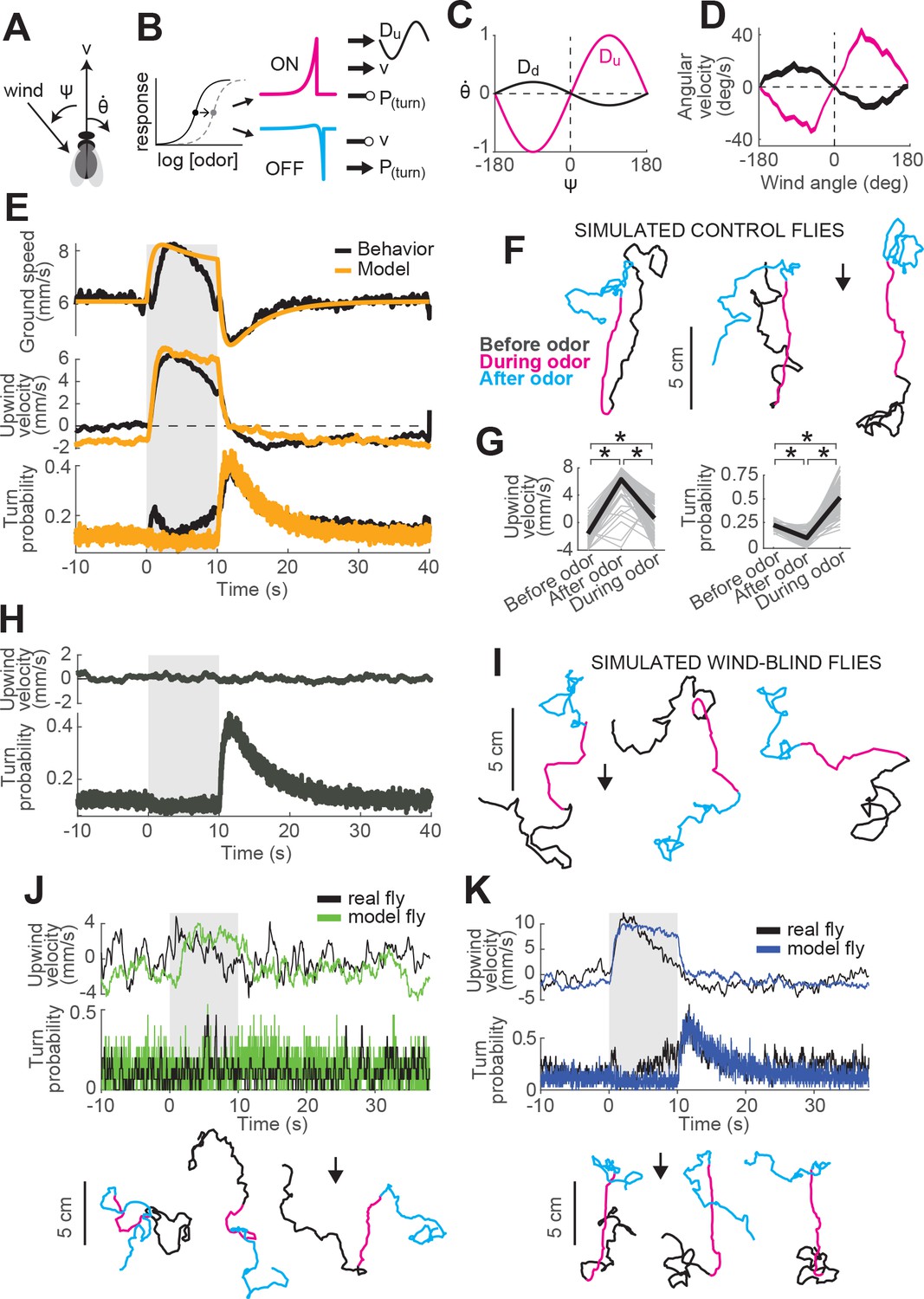
A navigation model based on ON and OFF functions can recapitulate many aspects of our behavioral data.
(A) Schematic of a fly showing model outputs (v: ground speed; : angular velocity) and input (: wind angle with respect to the fly). (B) Schematic of the model algorithm. Odor stimuli are first adaptively compressed, then filtered to produce ON (magenta) and OFF (cyan) functions. These functions modulate ground speed and angular velocity of the simulated fly. Angular velocity has both a stochastic component controlled through turn probability and a deterministic component guided by wind. (C) Wind direction influences behavior through two sinusoidal D-functions which drive upwind (magenta) and downwind (black) heading respectively. A weak downwind drive is always present, while a stronger upwind drive is gated by the ON function. (D) D-functions (average angular velocity as a function of wind angle with respect to the fly) calculated from responses of real flies (data from Figure 1, meanSEM, n = 75 flies, 1306 trials). Magenta trace: data from 0 to 2 s during odor. Black trace: 0–2 s after odor. (E–G) Simulated trajectories of model flies are similar to those of real flies. (E) Ground speed, upwind velocity and turn probability (average; n = 75 flies, 1306 trials) from real flies (black; data from Figure 1) and from 500 trials simulated with our model (orange) in response to a 10 s odor pulse. (F) Example trajectories from the simulation in E. Black: before odor. Magenta: during odor. Cyan: after odor. Black arrow: direction of the wind. (G) Mean values of upwind velocity and turn probability from the model simulations in E, before (−30 to 0 s), during (2 to 3 s) and after (11 to 13 s) the odor pulse. Gray lines: data from individual trials. Black lines: group average. Horizontal lines with asterisk: Statistically significant changes in a Wilcoxon signed rank paired test after correction for multiple comparisons using the Bonferroni method (see Materials and methods for p values). n.s.: not significant. (H–I) Simulated trajectories of wind-blind flies. (H) Upwind velocity and turn probability (average) from 500 trials simulated in response to a 10 s odor pulse with no wind (both D-functions coefficients set to 0) to mimic the responses of wind-blind flies (see Figure 2). Note the absence of modulation in upwind velocity. (I) Example trajectories from the simulation in H. Color code and arrow as in F. Note that trajectories preserve the characteristic shapes of the ON and OFF responses but lack any clear orientation during ON responses. (J–K) Simulated trajectories of weak and strong-searching flies. (J) Upwind velocity and turn probability of one weak-searching fly. Real fly appears in green-highlighted examples in Figure 1—figure supplement 2 (here black traces; average; n = 15 trials). The model simulation (green traces; average; n = 15 trials) was created by using the mean upwind velocity and turn probability for this fly (Figure 1—figure supplement 2, green) as a fraction of the population average upwind velocity and turn probability to scale the ON and OFF functions (values used: ON scale = 0.3, OFF scale = 0.26). Bottom: example trajectories from the model simulation, compare directly to Figure 1—figure supplement 2A left (color code and arrow as in F). (K) Equivalent to J, for one strong-searching fly (n = 34 trials). Compare blue-highlighted examples in Figure 1—figure supplement 2 with the model simulation (n = 34 trials; values used: ON scale = 1.9, OFF scale = 1.6).
Figure 6
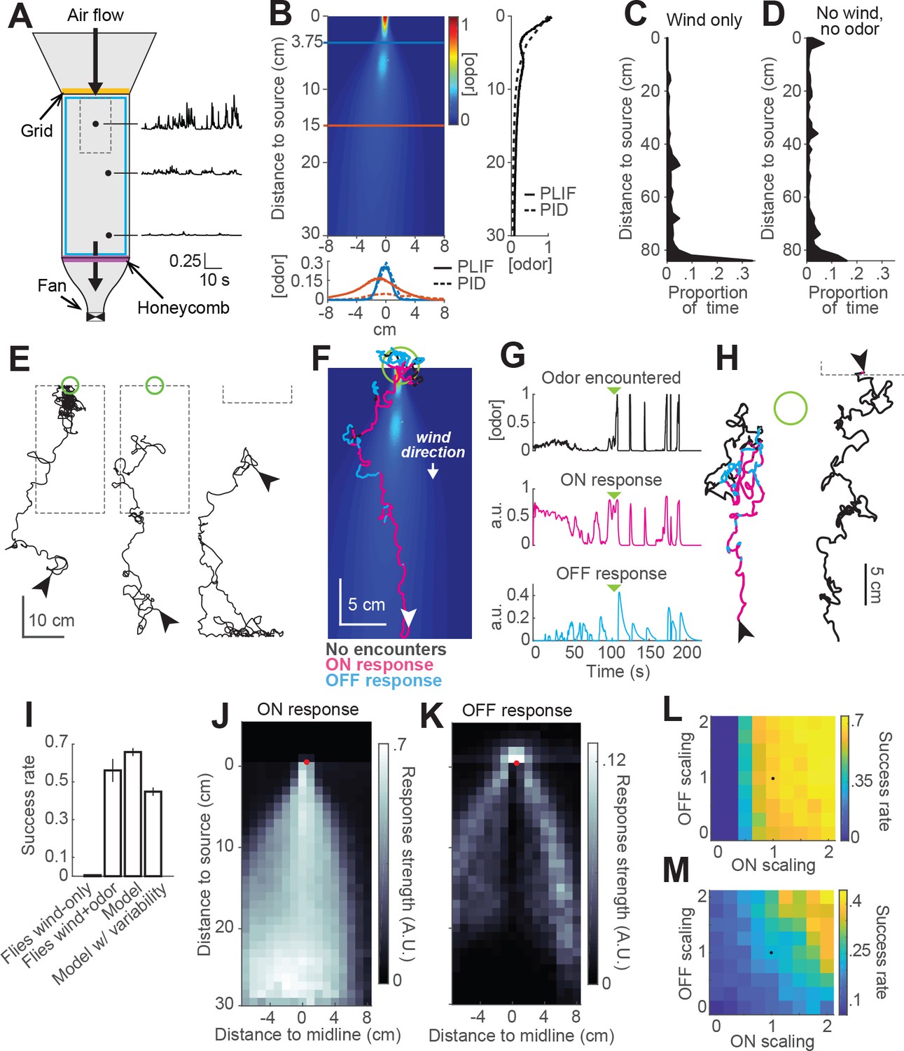
Real and virtual behavior of flies in a turbulent odor environment.
(A) Schematic of a turbulent wind tunnel used for behavioral experiments and PLIF imaging (top view; see Materials and methods). Black arrows: direction of air flow drawn by fan at downwind end; top arrow coincides with the tube carrying odor to the arena. Black dots and associated traces: sites of PID measurements (and corresponding signals; units normalized to mean concentration near the odor source). Smaller dashed square: Area covered with the PLIF measurements in the Colorado wind-tunnel (see Materials and methods). Yellow line: position of the wooden dowel grid. Purple line: position of the honeycomb filter. Blue square: perimeter moat filled with water. (B) PLIF measurements of an odor plume (average of 4 min of data). Blue/red horizontal lines: Sites of cross-sections (bottom plot). Bottom plot: cross-sections of the plume measured with PLIF (solid lines; 4 min average) and PID (dashed lines; 3 min average). Right plot: Odor concentration along midline of the plume (x = 0) measured with PLIF and PID (4 and 3 min average, respectively). All measurements in B appear normalized to average odor concentration at the source. (C–D) Flies exhibit a downwind preference in the turbulent wind tunnel. (C) Distribution of fly positions during trials with wind but no odor (n = 14 flies/trials). (D) Same as C, during trials with no wind (n = 13 flies/trials). (E) Example trajectories of flies during trials with an odor plume. From left to right: a successful trial in which the fly came within 2 cm of the source; intermediate trial in which the fly searched but did not find the source; failed trial where fly moved downwind. Arrowheads: starting positions. Green circles: 2 cm area around odor source. Dashed gray lines: area covered by PLIF measurements (use as positional reference; right-most trace shows only lower section of outline). (F) Example trajectory of a model fly that successfully found the odor source (background image from B). Colors show times when ON > 0.1 (magenta) or OFF > 0.05 (cyan). White arrowhead: Starting position and orientation. Green circle: 2 cm area around source. (G) Time courses of odor concentration encountered along the trajectory in F, with corresponding ON and OFF responses. Green arrowheads: time of entrance into the green circle. (H) Example trajectories of model flies (color code, green circle and arrowheads as in F). Left trace and green circle associated: intermediate trial where fly searched but did not find the source. Right trace: failed trial where fly moved downwind. Dashed line: lower section of the plume area. (I) Performance (proportion of successful trialsSE; see Materials and methods) of real and model flies in a plume. Data from real flies on trials with only wind (n = 13 flies/trials) and trials with wind and odor (n = 14 flies/trials). Model data using parameters fit to the mean fly in every trial (n = 500 trials; see Results). Model with variable ON and OFF scaling, reflecting variability in ON/OFF responses across individuals (n = 500 trials; see Results and Figure 1—figure supplement 2). (J–K) Average strength of ON (J) and OFF (K) responses as a function of position for model flies in the plume (data from simulation with mean parameters). Red dots: odor source. Note that ON is high throughout the odor plume, especially along its center, while OFF is highest at the plume edges. (L) Performance of the model in a plume (proportion of successful trials) with different scaling factors applied to ON and OFF responses. Black dot: performance of model using fitted values. (M) Same as L for model flies navigating a simulated odor gradient with a gaussian distribution and no wind (see Materials and methods).
Figure 7
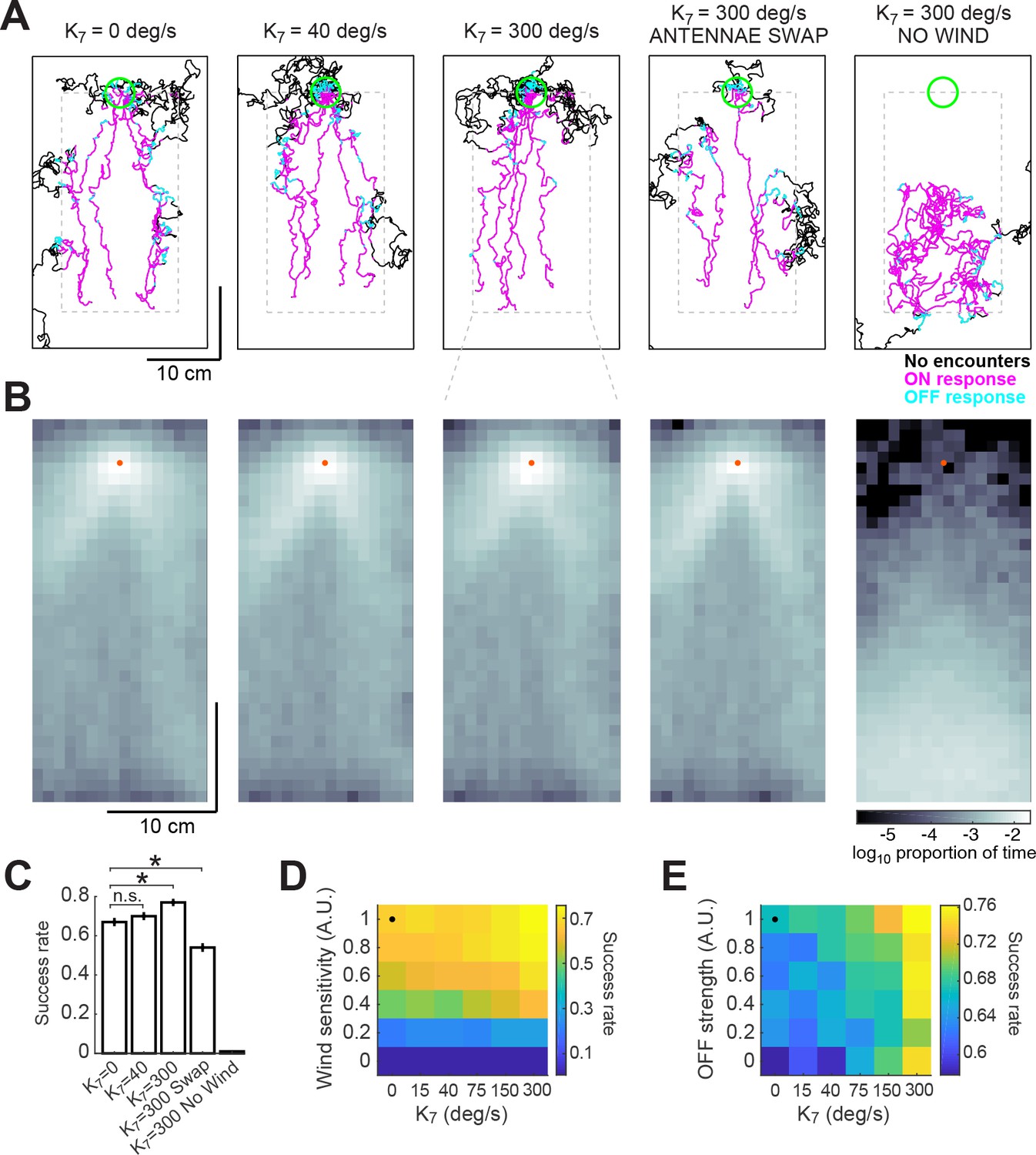
Addition of a bilateral sampling component can improve olfactory navigation.
(A) Example trajectories from a series of model simulations of 500 trials each. In the first simulation the model was unchanged (as in Figure 6). In the second and third simulations, a bilateral component was added to total angular velocity with gain values of 40 and 300 deg/s, respectively. In the fourth simulation, all components of the model were active, but the information from the antennae was swapped —left was interpreted as right, and vice-versa. In the fifth simulation, wind sensation was turned off. Trajectories’ colors show times when ON > 0.1 (magenta) or OFF >0.05 (cyan). Dashed gray lines: area of odor plume data (outside this area odor concentration is zero). A larger area is shown to display the behavior more clearly. Green circle: area of 2 cm around the odor source, used to define success in trials. (B) Density maps of flies’ positions (logarithm of the proportion of total time) corresponding to each of the simulations in A, with data only from the areas within the dashed lines in A. Orange dots: position of the odor source. (C) Success rate (proportion of successful trials) in each of the simulations in A (averageSEM; see Materials and methods). Horizontal lines with asterisk: Statistically significant changes (see Materials and methods for details and p values). n.s.: not significant. (D) Performance of the model in a plume (sucess rate) as a function of wind sensitivity and strength of the bilateral component. Note that values for don’t scale linearly. Black dot: performance of model using fitted values (see Results). (E) Equivalent to D, showing performance as a function of strength of the OFF response and of the bilateral component.
Author response image 1
Author response image 2

Videos
Video 1
Behavior of four flies in response to an ACV 10% pulse.
The time of the odor stimulus is signaled by the green dot appearing at the top of the image. Flies start to move upwind shortly after the start of the stimulus (partly due to the time it takes for the odor front to reach their respective positions), and they stop advancing upwind after the odor is gone and engage in a more localized search behavior. Air and odor move from the top of the image towards the bottom at 11.9 cm/s.
Video 2
Behavior of a model fly navigating an odor plume.
The video shows 3 min long trial, sped up four times. The background image represents the odor concentration of the plume (equivalent to Figure 6B) recorded by PLIF in the Colorado wind tunnel (see Materials and methods). The moving dot represents the position of the model fly, with changing colors depending on its current behavior. Magenta dot: ON response is larger than 0.1. Cyan dot: OFF response is larger than 0.05. White circle: no odor-evoked responses.
Tables
Table 1
Values of ON and OFF functions parameters.
Results of fitting the different ON and OFF functions to behavioral data by non-linear regression. Highlighted in green are the models of choice and the parameters that were used in the navigation model and the simulations shown in Figures 5 and 6. : different time constants of ON, OFF and adaptation filters. RMSE: root mean squared error between predictions of the models and the corresponding data they were fitted to. Corr.Coef.: Pearson’s linear correlation coefficients between predictions of the models and the corresponding data they were fitted to.
| ON MODEL | — | RMSE | Corr.Coef. | |||
|---|---|---|---|---|---|---|
| Filtering then adaptive compression (FAC) | 0.34 | — | 20.36 | 5.9 | 1.5784 | 0.89 |
| Adaptive compression then filtering (ACF) | 0.72 | — | 9.8 | 7.3 | 1.4122 | 0.92 |
| Filtering then compression (FC) | 0.04 | — | — | 4.4 | 1.747 | 0.85 |
| Compression then filtering (CF) | 0.3 | — | — | 4.5 | 1.7058 | 0.86 |
| OFF MODEL | RMSE | Corr.Coef. | ||||
| Filtering then adaptive compression (FAC) | 0.76 | 3.96 | 16.7 | 0.3 | 0.0345 | 0.75 |
| Adaptive compression then filtering (ACF) | 0.62 | 4.84 | 10.08 | 0.6 | 0.0336 | 0.77 |
| Filtering then compression (FC) | 0.58 | 3 | — | 0.1 | 0.0409 | 0.62 |
| Compression then filtering (CF) | 0.06 | 5.02 | — | 0.3 | 0.0389 | 0.69 |
Table 2
Values of navigation model parameters used in all simulations in this article, with their function in the model explained.
https://doi.org/10.7554/eLife.37815.014| Navigation model | |||
|---|---|---|---|
| Parameter | Value | Units | Role |
| 0.12 | Rate | Baseline turn rate | |
| 20 | deg/s | Standard deviation of angular velocity distribution | |
| 6 | mm/s | Baseline ground speed | |
| 0.45 | mm/s | Strength of ON speed modulation | |
| 0.8 | mm/s | Strength of OFF speed modulation | |
| 0.03 | — | Strength of ON turning modulation | |
| 0.75 | — | Strength of OFF turning modulation | |
| 5 | deg/sample | Strength of ON upwind-drive modulation | |
| 0.5 | deg/sample | Strength of downwind-drive modulation | |
Key resources table
| Reagent type or resource | Designation | Source or reference | Identifiers | Additional information |
|---|---|---|---|---|
| Gene (Drosophila melanogaster) | norpA36 | NA | FLYB:FBgn0262738 | — |
| Genetic reagent (Drosophila melanogaster) | w1118 norpA36 | This paper | FLYB:FBal0013129 | Progenitor = norpA36 obtained from C. Desplan; backcrossed 7 generations to Bloomington stock 5905 = w1118 |
Additional files
-
Transparent reporting form
- https://doi.org/10.7554/eLife.37815.018
Download links
A two-part list of links to download the article, or parts of the article, in various formats.
Downloads (link to download the article as PDF)
Open citations (links to open the citations from this article in various online reference manager services)
Cite this article (links to download the citations from this article in formats compatible with various reference manager tools)
Elementary sensory-motor transformations underlying olfactory navigation in walking fruit-flies
eLife 7:e37815.
https://doi.org/10.7554/eLife.37815


