Figures and data in Variance adaptation in navigational decision making

Figures
Tables
Additional files

9 figures, 2 tables and 1 additional file

Figures

Figure 1 with 2 supplements

Download asset Open asset

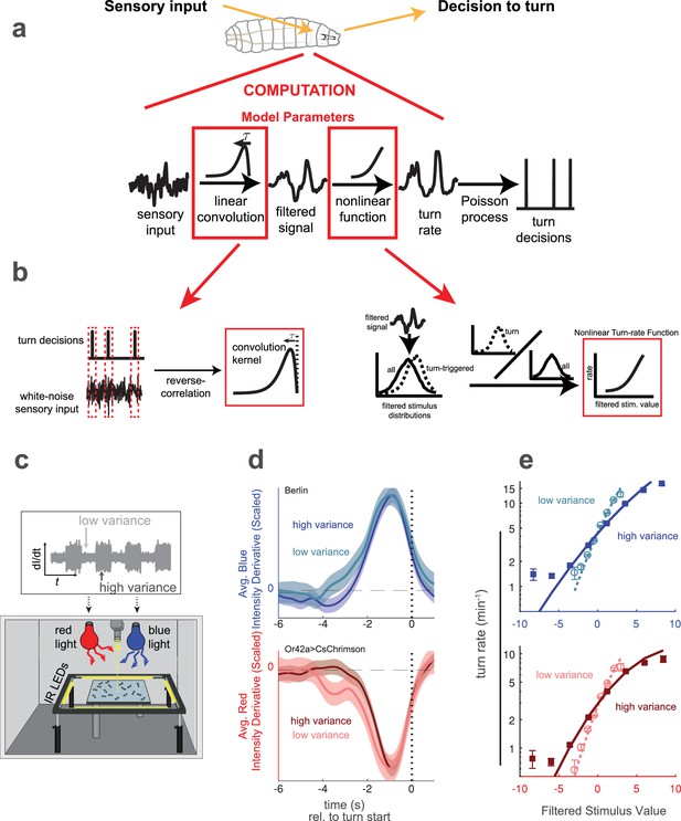
Reverse correlation analysis of variance adaptation.

(a) Linear-Nonlinear-Poisson (LNP) model of the decision to turn. Sensory input is processed by a linear filter to produce an intermediate signal. The rate at which the larva initiates turns is a nonlinear function of this signal. Turns are initiated stochastically according to a Poisson process with this underlying turn rate. (b) Reverse correlation to determine LNP model parameters. The kernel of the linear filter is proportional to the 'turn-triggered-average', the average input preceding turns. The rate function is calculated by comparing the turn-conditioned filtered inputs to the entire input ensemble. (c) Experimental setup to test for behavioral adaptation to variance. We presented fluctuating light intensities - with randomly-picked derivatives - to groups of larvae crawling on an agar surface, and recorded their trajectories using IR lights and camera. Blue light provided a visual stimulus and red light activation of CsChrimson labeled neurons provided a fictive olfactory stimulus. The derivative of the light intensity was the input to our LNP model, and the variance of this input periodically changed between low and high values. (d) Turn-triggered averages measured at low and high variances for visual (Berlin, blue light) and fictive attractive odor (Or42aCsChrimson, red light) stimuli. To ease comparison of the temporal structure, the averages are scaled to have the same peak value. (e) Nonlinear rate functions measured at low and high variances. A single convolution kernel was calculated for the entire experiment; the turn rate as a function of the filtered input was calculated separately for low and high variance. Note logarithmic y-axis. *Number of experiments, animals in* Table 1.

https://doi.org/10.7554/eLife.37945.002

Figure 1—figure supplement 1

Download asset Open asset

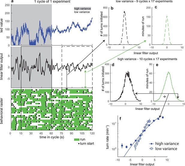
Overview of analysis steps.

Overview of analysis steps Graphical demonstration of the calculation of the visual rate functions in Figure 1e (a) Example data from 1 cycle of one visual variance adaptation experiment. Top: led output value vs. time - 0 is off and 255 is max intensity. Middle: convolution of derivative of led output value with linear filter found via reverse correlation. Bottom: behavioral raster - each row represents one larva. Green shaded regions indicate larva was in a run, black circles represent turn initiations. Solid box indicates data used to compute high variance rate function. Dashed line indicates data used to compute low variance rate function. (b) Histogram of convolved stimulus values at the instant a turn was initiated, at low variance, for entire data set. (c) Histogram showing amount of time larva was in a run and therefore capable of initiating a turn vs. convolved stimulus, at low variance, for entire data set. Arrows show how elements of these histograms are extracted from the data. (d) Histogram of convolved stimulus values at the instant a turn was initiated, at high variance, for entire data set. (e) Histogram showing amount of time larva was in a run vs. convolved stimulus, at high variance, for entire data set. (f) Turn rate vs. convolved stimulus for high and low variance. Markers indicate rate found by dividing number of turns by minutes of run. Lines are maximum likelihood estimates of rate functions given convolved stimulii and observed behaviors.

https://doi.org/10.7554/eLife.37945.003

Figure 1—figure supplement 2

Download asset Open asset

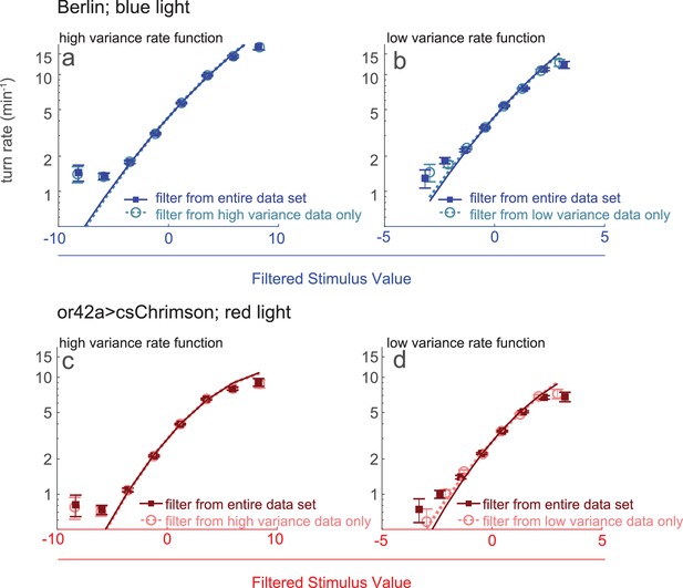
Rate functions following single filter vs variance-specific filters.

Rate functions following single filter vs. variance-specific filters Rate functions of Figure 1e re-calculated using filters derived from high and low variance turn-triggered averages. (**a,b**) Berlin larvae responding to blue light. Rate functions at (a) high or (b) low variance calculated using either a filter derived from the entire data set (Figure 1e) or a filter derived from the turn-triggered average at high or low variance only. Note logarithmic y-axis, different x-axes. (**c,d**) Or42a>csChrimson larvae responding to red light. Rate functions at (c) high or (d) low variance calculated using either a filter derived from the entire data set or a filter derived from the turn-triggered average at high or low variance only. Note logarithmic y-axis, different x-axes.

https://doi.org/10.7554/eLife.37945.004

Figure 2

Download asset Open asset

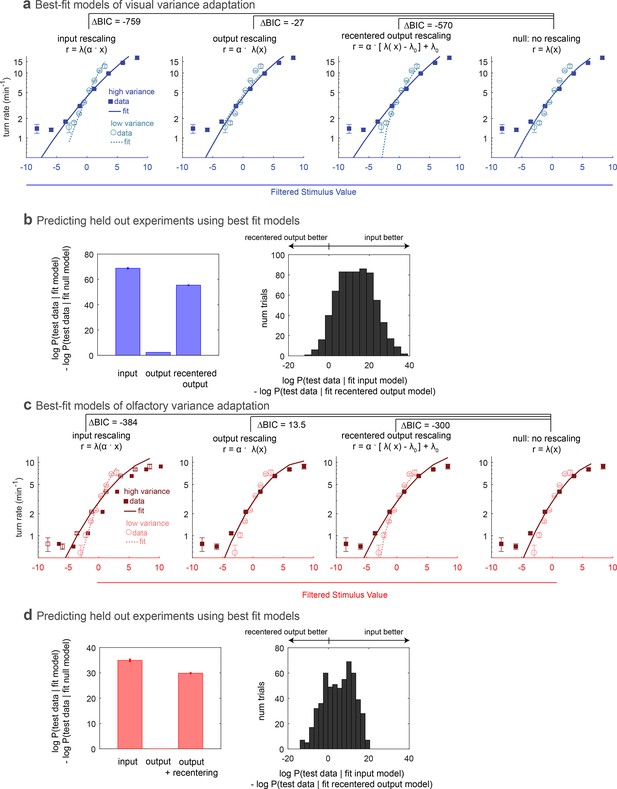
Comparing rescaling models of variance adaptation.

(a) Best fit rate functions to visual (Berlin with blue light stimulus) data of Figure 1, for various functional forms of rescaling, and for a null model with no rescaling. $Δ B I C$ indicates difference in Bayes Information Criterion between the adapting model and the null model. A negative value indicates the adapting model is preferred, and a difference of more than 10 is considered to be highly significant. (**b,c**) Ability of models to predict held-out data. In repeated ‘trials,’ each model was fit to a subset (14/17 experiments) of the data. The fit model was applied to calculate the likelihood of the data in the held out sets. Because test data sets varied in size, the log likelihood of each data set was normalized to the mean length of all test data sets. (b) Increase in log-likelihood of test data when predicted with rescaling models over the predictions of a null model without rescaling. Bars show mean increase and error bars the standard error of the mean. (c) Histogram of improvement of input rescaling model predictions over recentered output rescaling model predictions for each ‘trial.’ $Δ$ log-likelihood $>$ 4.6 corresponds to $p < 0.01$ . (**d–f**) Same as (**a–c**), but for fictive olfactory (Or42a>csChrimson with red light stimulus) data of panel 1. *Number of experiments, animals in* Table 1

https://doi.org/10.7554/eLife.37945.005

Figure 3

Download asset Open asset

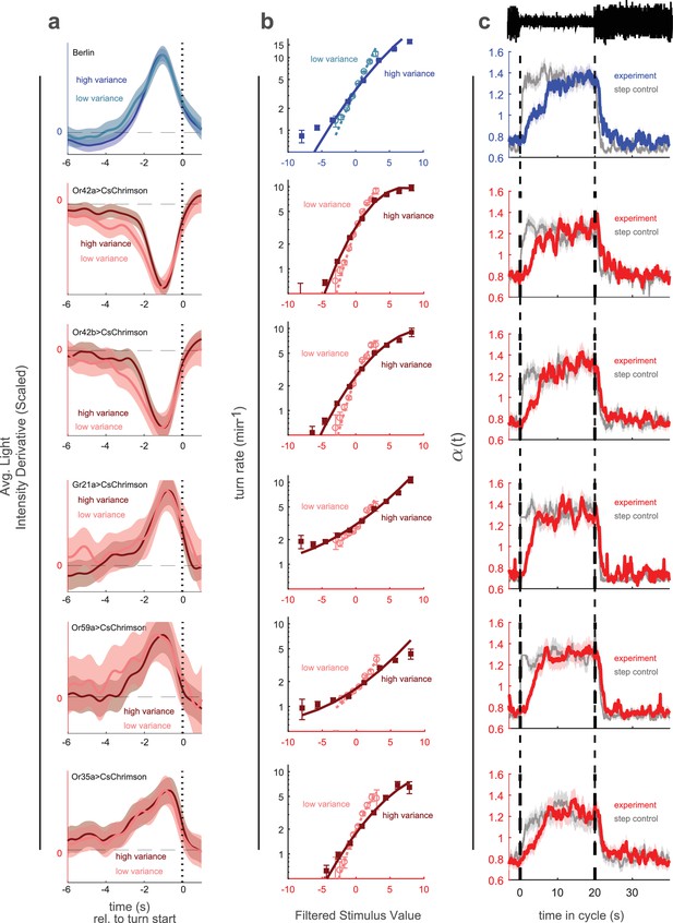
Variance adaptation and temporal dynamics of input rescaling.

Larvae were exposed to alternating 20 s periods of high and low variance intensity derivative white noise. For Berlin, the stimulus was visual (blue light). For all other genotypes, the stimulus was optogenetic activation of the indicated receptor neuron type via CsChrimson and red illumination. (a) Turn-triggered averages measured at low and high variances. To ease comparison of the temporal structure, the averages are scaled to have the same peak value. (b) Nonlinear rate functions measured at low and high variances. A single convolution kernel was calculated for the entire experiment; the turn rate as a function of the filtered stimulus was calculated separately for low and high variance. Note logarithmic y-axis. (c) Scaling factor ( $α (t)$ ) vs. time since switch to low variance, averaged over many cycles. Schematic at top indicates low and high variance conditions. Colored lines (experiment) are maximum likelihood fits to data. Gray lines (step control) are maximum likelihood fits to data generated by a model in which the input rescaling changes instantly when the variance changes. $α$ was normalized so that the average over the entire experiment was 1. *Number of experiments, animals in* Table 1

https://doi.org/10.7554/eLife.37945.006

Figure 4 with 1 supplement

Download asset Open asset

Variance adaptation to a stimulus with uncorrelated values.

Berlin wild type animals were exposed to blue light. Every 0.25 s, the intensity of the light was chosen from a random normal distribution with fixed mean and low or high variance. (a) Turn-triggered average deviation from mean intensity, scaled to have same peak value at high and low variance. Analogous to Figure 1d. (b) Nonlinear rate functions measured at low and high variances. A single convolution kernel was calculated for the entire experiment; the turn rate as a function of the filtered input was calculated separately for low and high variance. Note logarithmic y-axis. Analogous to Figure 1e. (c) Scaling factor ( $α (t)$ ) vs. time since switch to low variance, averaged over many cycles. Colored lines (experiment) are maximum likelihood fits to data. Gray lines (step control) are maximum likelihood fits to data generated by a model in which the input rescaling changes instantly when the variance changes. $α$ was normalized so that the average over the entire experiment was 1. Analogous to Figure 3c. *Number of experiments, animals in* Table 1.

https://doi.org/10.7554/eLife.37945.007

Figure 4—figure supplement 1

Download asset Open asset

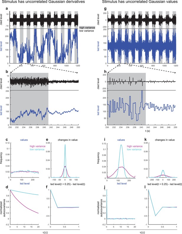
Comparison of stimulii with uncorrelated random derivatives and uncorrelated random values.

Comparison of stimulii with uncorrelated random derivatives and uncorrelated random values Left: uncorrelated random derivatives. (a) Light levels (blue, below) and difference between subsequent light levels in light levels (black, above) vs. time for a single experiment. High variance periods are shaded in gray. Light levels range from 0 (fully off) to 255 (maximum intensity). (b) Zoomed in portion of trace in (a) showing transition from high to low variance. (c) Histogram of light levels over entirety of data used to produce Figure 1, separated into high and low variance portions (d) Normalized autocovariance of light levels for entire data set, separated into high and low variance portions. (e) Histogram of changes between light levels separated by 0.25 s, separated into high and low variance portions. (f) Normalized autocovariance of light level changes, separated into high and low variance portions. Right: uncorrelated random values. (g) Light levels (blue, below) and difference between subsequent light levels in light levels (black, above) vs. time for a single experiment. High variance periods are shaded in gray. Light levels range from 0 (fully off) to 255 (maximum intensity). (h) Zoomed in portion of trace in (g) showing transition from high to low variance. (i) Histogram of light levels over entirety of data used to produce Figure 4, separated into high and low variance portions (j) Normalized autocovariance of light levels for entire data set, separated into high and low variance portions. (k) Histogram of changes between light levels separated by 0.25 s, separated into high and low variance portions. (l) Normalized autocovariance of light level changes, separated into high and low variance portions. Note that in a,b,g,h changes in light levels are calculated every 8 ms, the actual update rate of the apparatus. In e,f,k,l changes in light levels are calculated every 250 ms, the update rate of the random value experiments.

https://doi.org/10.7554/eLife.37945.008

Figure 5

Download asset Open asset

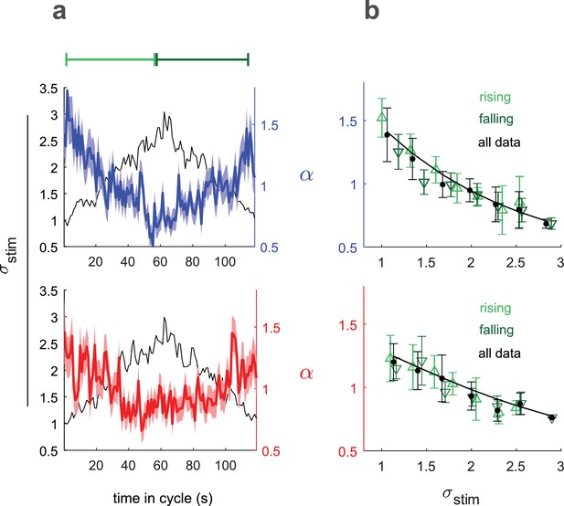
Input rescaling as a function of variance.

Larvae were exposed to intensity derivative white noise whose standard deviation steadily increased and decreased in a 120 s period triangle wave. Top row: visual stimulus - blue light was presented to Berlin wild type. Bottom row: fictive attractive odor stimulus - red light activated CsChrimon expressed in Or42a receptor neurons. (a) Rescaling factors ( $α$ ) and stimulus standard deviation ( $σ$ ) vs. time since variance started increasing. (b) Rescaling factor ( $α$ ) vs. stimulus standard deviation, as calculated from data in (a). Rising, falling indicate $α$ vs. $σ$ calculated using only data when variance was increasing or decreasing respectively. Solid black line is a fit to Equation 3 using all data. *Number of experiments, animals in* Table 1

https://doi.org/10.7554/eLife.37945.009

Figure 6

Download asset Open asset

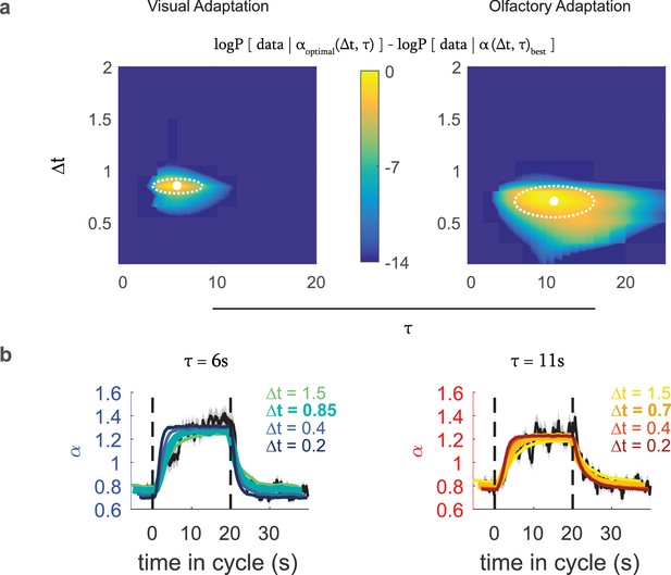
Optimal variance estimator predicts input rescaling.

We generated an estimate of the input variance using a Bayes estimator that sampled the stimulus at an interval of $Δ t$ , with a prior $τ$ that represented the expected correlation time of environmental variance, which we converted to an input rescaling parameter using the relation found in Figure 5. We found the static rate function parameters that in combination with this rescaling parameter best predicted the actual experimental data. We repeated this process for various combinations of $Δ t$ and $τ$ to find the one that best modeled the experimental data (a) Difference from the optimal log likelihood of data given model for various choices for $Δ t$ , $τ$ , for the visual and fictive olfactory (Or42a $>$ CsChrimson) variance switching experiments of Figure 3. (b) Measured (black line) and predicted (colored lines) input rescaling vs. time for variance switching experiments, for the best fit value of $τ$ and varying values of $Δ t$ . The thickest colored line is the prediction of the best-fit estimator. *Number of experiments, animals in* Table 1

https://doi.org/10.7554/eLife.37945.010

Figure 7

Download asset Open asset

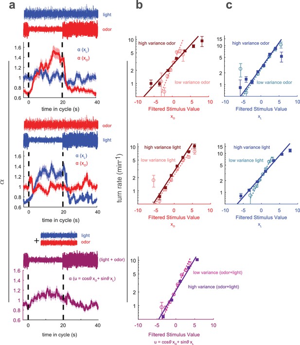
Multisensory variance adaptation and temporal dynamics of input rescaling.

Or42a $>$ CsChrimson larvae were exposed to both visual (dim blue light) and fictive olfactory (red light) stimuli with random intensity derivatives. *Top row*: visual input had constant variance, while olfactory input alternated between high and low variance every 20 s. *Middle row*: Olfactory input had constant variance and visual input alternated between high and low variance. *Bottom row*: Both olfactory and visual inputs had constant variance, but alternated between correlated and anti-correlated every 20 s. (a) Estimated input rescaling vs. time since variance switched to low, averaged over many cycles, for light and odor (top two rows) or combinations of light and odor (bottom row). (b) Turn rate vs. output of odor filter at high and low variance of the switching stimulus (top two rows) and vs. a linear combination of light and odor (bottom row). (c) Turn rate vs. output of light filter at high and low variance of the switching stimulus (top two rows). Note logarithmic y-axis in b,c. *Number of experiments, animals in* Table 1

https://doi.org/10.7554/eLife.37945.011

Figure 8 with 2 supplements

Download asset Open asset

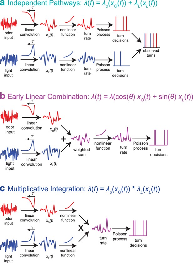
Multisensory combination models.

(a) Indepdendent pathways: two independent LNP models transform odor and light stimuli into decisions to turn; these turn decisions are combined by an OR operation at a late stage. This model is inconsistent with data from multisensory white noise experiments. (b) Early linear combination: Filtered odor and light signals are combined via linear summation prior to nonlinear transformation of the combined signal. This model is difficult to reconcile with adaptation to variance on a single-sense basis. (c) Multiplicative integration: Separate LN models for odor and light are combined via multiplication of the nonlinear function outputs. This model allows for unisensory variance adaptation via rescaling of a rectifying nonlinearity and is consistent with data from multisensory white noise experiments. Adapted from Gepner et al. (2015).

https://doi.org/10.7554/eLife.37945.012

Figure 8—figure supplement 1

Download asset Open asset

Reanalysis of white noise experiments.

Reanalysis of white noise experiments (a) Results from Gepner et al. (2015). Left: turn-triggered average changes in visual stimulus (blue) and optogenetic activation (red) for entire data set. These were used to create the kernels for the linear convolution stage. Center: Turn-triggered ensemble - two-dimensional histogram of odor and light filter outputs at the moment of turn initiation. Right: rotated coordinate system; all turning decisions were described as a function of $u$ , a linear combination of light and odor filter outputs. (b) Turn-triggered ensembles predicted by the best fit independent pathways, early linear combination, and multiplicative integration models to the entire data set. $Δ B I C$ indicates difference in Bayes Information Criterion between the left and right models. A negative value indicates the right model is preferred, and a difference of more than 10 is considered to be highly significant. By eye it is difficult to see a difference between the predictions of the multiplicative and linear combination models; the predicted turn-triggered ensembles differ by $\leq 10 %$ in the high probability regions. (c) Testing the predictions of the three models against held-out data. 9/12 experiments were used to fit the models and these fits were used to predict the turn rate in the held out three experiments. Left: Improvement in log-likelihood of test data given fit model over prediction of null model (fit to mean turn rate only) for all three models. Mean and standard error of mean are shown. The size of the error bars is due to mainly to sensitivity of the null model predictions to differences in the mean turn rate of the predicted and test data sets. Right: histogram of improvement of multiplicative integration over early linear combination, for each permutation of fit and test data (220 total). Because test data sets varied in size, the log likelihood of each data set was normalized to the mean length of all test data sets. Data from Gepner et al. (2015), which contains information on the number of experiments, larvae, and turns.

https://doi.org/10.7554/eLife.37945.013

Figure 8—figure supplement 2

Download asset Open asset

Reanalysis of multisensory step experiments.

Reanalysis of multisensory step experiments Measured and fit turn rate for various combinations of favorable and unfavorable changes in odor and light stimuli. $Δ B I C$ indicates difference in Bayes Information Criterion between the top and bottom models. A negative value indicates the lower model is preferred, and a difference of more than 10 is considered to be highly significant. Figure adapted from Gepner et al. (2015), which contains information on the number of experiments, larvae, and turns.

https://doi.org/10.7554/eLife.37945.014

Figure 9

Download asset Open asset

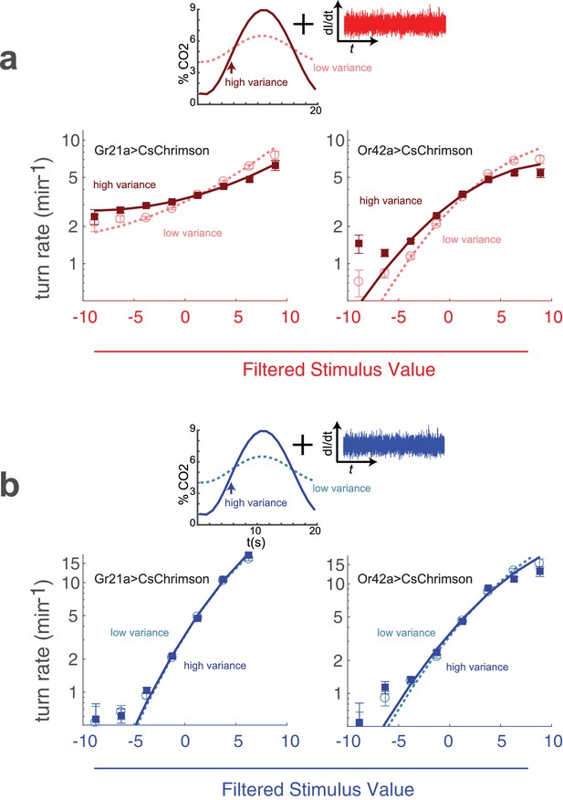
Adaptation to variance in a natural odor background.

(a) Optogenetic activation of odor receptor neurons with a fluctuating background of carbon dioxide. Above: Noise of constant variance was provided to either the CO $_{2}$ receptor neuron (Gr21a $>$ CsChrimson) or an Ethyl Acetate receptor neuron (Or42a $>$ CsChrimson) in a flow chamber with a time-varying CO $_{2}$ concentration. The mean CO $_{2}$ concentration was 5% in both high and low variance conditions, but the amplitude of the fluctuation was larger in the high variance condition. Below: turn rate as a function of filtered stimulus for both high and low variance conditions. Note logarithmic y-axis. (b) Visual stimulus with a fluctuating background of carbon dioxide. The same as (a) but the stimulus was blue noise of constant variance. *Number of experiments, animals in* Table 1

https://doi.org/10.7554/eLife.37945.015

Tables

Key resources table

Reagent type (species) or Resource	Designation	Source or reference	Identifiers
Strain (Drosophila melanogaster)	Berlin wild type	gift of Justin Blau, NYU
Genetic reagent (D. melanogaster)	w1118;;20XUAS- CsChrimson-mVenus	Bloomington Stock Center	RRID:BDSC_55136
Genetic reagent (D. melanogaster)	w*;;Gr21a-Gal4	Bloomington Stock Center	RRID:BDSC_23890
Genetic reagent (D. melanogaster)	w*;;Or42a-Gal4	Bloomington Stock Center	RRID:BDSC_9969
Genetic reagent (D. melanogaster)	w*;;Or42b-Gal4	Bloomington Stock Center	RRID:BDSC_9972
Genetic reagent (D. melanogaster)	w*;;Or35a-Gal4	Bloomington Stock Center	RRID:BDSC_9968
Genetic reagent (D. melanogaster)	w*;;Or59a-Gal4	Bloomington Stock Center	RRID:BDSC_9989
Software, algorithm	MAGATAnalyzer	(Gershow et al., 2012) github.com/samuellab/MAGATAnalyzer-Matlab-Analysis/	d9d72b2b43c82af...

Table 1

Number of experiments, animals, turns.

# experiments - number of 20 min duration experiments; a different noise input was used for each experiment within a group; # animals - estimate of total number of individual larvae surveyed in each set; animal-hours - total amount of animal-time analyzed; # turns total number of turns observed

https://doi.org/10.7554/eLife.37945.016

Figure	Genotype	# expts	# animals	animal-hours	# turns
Figure 1,Figure 2	Berlin	17	811	219.3	48711
Figure 1,Figure 2	Or42a $>$ CsChrimson	17	743	201.1	33822
Figure 3	Berlin	30	1087	302.4	55776
	Or42a $>$ CsChrimson	19	838	247.5	44806
	Or42b $>$ CsChrimson	15	600	163.3	23826
	Or59a $>$ CsChrimson	15	723	177.6	16418
	Or35a $>$ CsChrimson	11	430	121.1	13149
	Gr21a $>$ CsChrimson	19	786	230.1	36121
Figure 4a,b	Berlin	16	483	133	22741
Figure 4c	Berlin	18	699	189	28226
Figure 5	Berlin	10	372	102.5	18397
Figure 5	Or42a $>$ CsChrimson	13	553	147.2	21897
Figure 7	Or42a $>$ CsChrimson
Odor switches variance, visual constant		6	165	46.1	6772
Odor constant variance, visual switches		10	391	105.4	15210
Correlation switches		16	616	156.8	22142
Figure 9a	Gr21a $>$ CsChrimson
High Variance CO $_{2}$		6	242	66.2	11286
Low Variance CO $_{2}$		6	242	62.4	10534
Figure 9a	Or42a $>$ CsChrimson
High Variance CO $_{2}$		7	286	80.5	12976
Low Variance CO $_{2}$		7	276	77.9	12096
Figure 9b	Gr21a $>$ CsChrimson
High Variance CO $_{2}$		3	121	33.2	7289
Low Variance CO $_{2}$		3	116	32.7	7023
Figure 9b	Or42a $>$ CsChrimson
High Variance CO $_{2}$		2	94	25	5174
Low Variance CO $_{2}$		2	82	22.4	4571