Environmental deformations dynamically shift the grid cell spatial metric
Figures
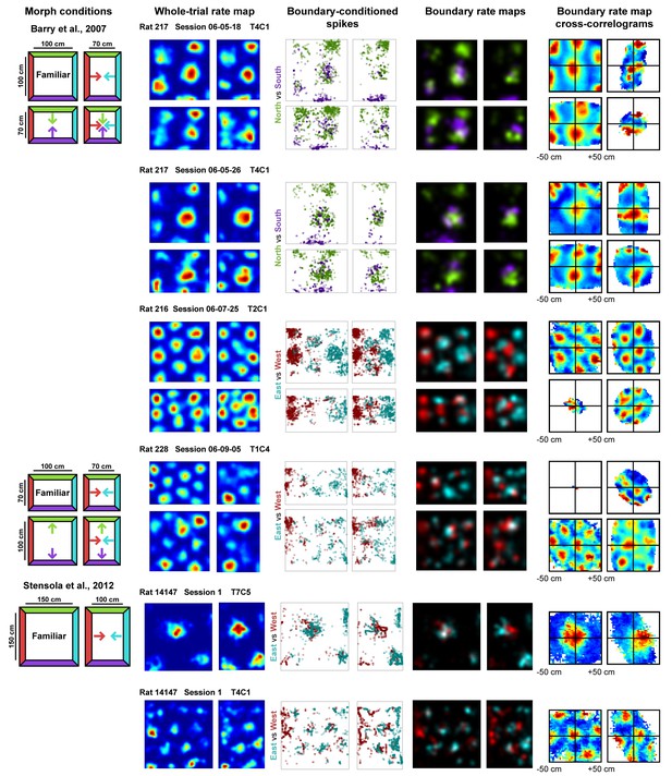
Examples of whole trial rate maps, boundary-conditioned spikes, boundary rate maps, and cross-correlograms of opposing boundary rate maps for recorded grid cells.
Rat, session, and cell identity indicated above whole trial rate maps. Boundary-conditioned spikes and boundary rate maps organized by opposing north-south (green—purple) and east-west (blue—red) boundary pairs. Colored arrows in morph condition indicate the shifts predicted by the boundary-tethered model during each deformation.

Opposing boundary rate maps are relatively shifted in phase along deformed dimensions during deformations.
Data from all experiments in (Barry et al., 2007; Stensola et al., 2012) combined. All error bars denote mean ±SEM. (A) Grid shift as measured by the relative phase between opposing boundary rate maps along deformed and undeformed dimensions. Because of the periodic nature of the grid pattern, shift is bounded by one half of the grid scale. Therefore, we quantify shift as a ratio of shift / (scale/2). (paired t-tests, 1st familiar vs. deformed: t(80) = 5.44, p<0.001; undeformed vs. deformed: t(83) = 4.21, p=0.001; 2nd familiar vs. deformed: t(82) = 5.07, p<0.001; all other comparisons: t < 1.10, p>0.2731; Figure 2—source data 1). (B) Histogram of grid scale (left) and shift ratio separated by grid scale along deformed dimensions with mean familiar shift ratio subtracted (right). (t-test versus 0, scale <60 cm: t(45) = 3.43, p=0.001; scale >60 cm: t(40) = 4.67, p<0.001; Figure 2—source data 1). (C) Histogram of rescaling (left) and shift ratio separated by rescale along deformed dimensions with mean familiar shift ratio subtracted (right). Because rescaling could vary within cell along deformed dimensions, each condition and deformed dimension was treated independently. (t-test versus 0, rescaling <50%: t(61) = 3.39, p=0.001; rescaling >50%: t(130) = 7.05, p<0.001; Figure 2—source data 1). **p<0.01, ***p<0.001.
-
Figure 2—source data 1
Results of grid shift analyses.
Contains the values resulting from the shift analysis for each cell trial, as well as the familiar grid scale, amount of rescaling, and shuffled control shift on each trial for each cell.
- https://doi.org/10.7554/eLife.38169.005
-
Figure 2—source data 2
Results of phase alignment analysis.
Contains the values resulting from the alignment analysis indicating whether each boundary rate map was best aligned with the familiar rate map by the most recently contacted boundary (1) or the opposing boundary (0).
- https://doi.org/10.7554/eLife.38169.006
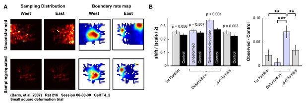
Controlling for sampling biases when measuring boundary-tethered shift.
To control for sampling differences following each boundary contact during each trial, we matched the sampling distributions of opposing boundary rate maps when computing shift. (A) Example sampling distributions and boundary rate maps when all data following boundary contacts are included (top row) and when the sampling distributions are equated (bottom row). (B) Because the deformed environments differ in shape and size from the familiar environments, and because the particular movement trajectories of the animal differ from trial to trial, there may be differences in the baseline amount of shift one would expect to observe across conditions. To control for this possibility, we used the whole-trial rate map of each cell as a template for simulating Poisson spikes using the same trajectory as the recorded data. From these simulations, we extracted boundary tethered rate maps and computed shifts between maps tethered to opposite boundaries. We repeated this process 100 times, and took the mean as our measure of the shift one would expect by chance for a cell with that particular rate map and sampling trajectory. This control reflects the shift one would expect if each boundary rate map were a random draw from a stable whole-trial rate map. The shift observed along deformed dimensions exceeded this control (paired t-test: t(87)=5.67, p<0.001). Moreover, the difference between the observed and control shift values was significantly larger along deformed dimensions than that of all other conditions (paired t-tests, 1st familiar vs. deformed: t(80) = 2.66, p=0.010; undeformed vs. deformed: t(83) = 3.77, p<0.001; 2nd familiar vs. deformed: t(82) = 2.64, p=0.010; all other comparisons: t < 1.9, p>0.060; Figure 2—source data 1).
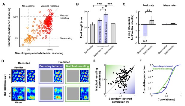
Additional tests of boundary-tethered phase shift predictions.
Data from all experiments in (Barry et al., 2007; Stensola et al., 2012) combined unless otherwise noted. All error bars denote mean ± SEM. All reported statistics are paired t-tests, unless otherwise noted. (A) Whole-trial versus boundary-conditioned grid rescaling factors, normalized to range from no rescaling (0%) to a matched rescaling (100%). Boundary-conditioning resulted in a significant reduction in the appearance of rescaling (t(194) = 9.54, p<0.001; Figure 3—source data 1). (B) Field length along deformed and undeformed dimensions during compression deformations. (1st familiar vs. deformed: t(80) = 3.70, p<0.001; undeformed vs. deformed: t(86) = 2.43, p=0.017; 2nd familiar vs. deformed: t(82) = 3.49, p<0.001; all other comparisons: t < 1.45, p>0.151; Figure 3—source data 2). (C) Change in firing rates across conditions. (Peak firing rates, 1st familiar vs. deformation: t(80) = 3.57, p<0.001; 2nd familiar vs. deformation: t(82) = 3.34, p=0.001; 1st familiar vs. 2nd familiar: t(76) = 0.91, p=0.364; Mean firing rates, 1st familiar vs. deformation: t(80) = 3.57, p<0.001; 2nd familiar vs. deformation: t(82) = 3.34, p=0.001; 1st familiar vs. 2nd familiar: t(76) = 0.91, p=0.364; Mean firing rates, 1st familiar vs. deformation: t(80) = 0.54, p=0.591; 2nd familiar vs. deformation: t(82) = 0.03, p=0.978; 1st familiar vs. 2nd familiar: t(76) = 0.71, p=0.479; Figure 3—source data 3). (D) Examples of recorded and predicted rate maps during one deformation trial for two simultaneously recorded cell from (Stensola et al., 2012). (E) Correlation values between the recorded rate map and the rate maps predicted by the boundary-tethered model versus a matched rescaling during compression deformations (Figure 3—source data 4). (F) Cumulative distribution of the correlation values depicted in (E). The boundary-tethered model results in fewer low-similarity predictions than a matched rescaling (two-sample Kolmogorov-Smirnov test: D = 0.2030, p=0.007: Figure 3—source data 4). *p<0.05, **p<0.01, ***p<0.001.
-
Figure 3—source data 1
Results of rescaling analysis.
Contains the values resulting from the rescaling analysis indicating for each deformed axis the amount of rescaling observed during the whole trial, after boundary-conditioning, and when only a subset of the whole-trial data are included to match the boundary-conditioned sampling distribution.
- https://doi.org/10.7554/eLife.38169.009
-
Figure 3—source data 2
Results of field length analysis.
Contains the values resulting from the field length analysis in pixels for each cell.
- https://doi.org/10.7554/eLife.38169.010
-
Figure 3—source data 3
Results of firing rate analysis.
Contains the values resulting from the firing rate analysis in Hertz for each cell.
- https://doi.org/10.7554/eLife.38169.011
-
Figure 3—source data 4
Results of map prediction analysis.
Contains the correlation values between the recorded deformation trial rate map and the rate maps predicted by the boundary-tethered model and a matched rescaling for each cell and trial.
- https://doi.org/10.7554/eLife.38169.012
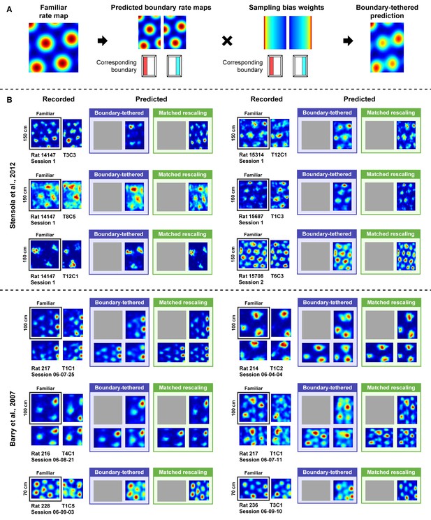
Predicting whole-trial rate maps from boundary-tethered shifts in grid phase.
(A) To predict rate maps from the boundary-tethered shifts for each cell and compression deformation trial we first created predicted boundary rate maps from the familiar environment rate map for each displaced boundary. These rate maps were shifted versions of the familiar rate map, aligned by the corresponding boundary. If the length of a boundary changed, then the central portion of the familiar rate map was used to construct the boundary rate map. Next, the contribution of each boundary rate map at each location was weighted by the actual probability of sampling that location following contact with the corresponding boundary for that deformation trial, computed from the actual path of the rat during that deformation trial. The final boundary-tethered prediction was then the smoothed sum of these predicted boundary rate maps. (B) Example recorded rate maps, accompanied by the predictions from the boundary-tethered model and a rescaling matched to the extent of the deformation. Rat, session, and cell identity indicated below each set of recorded rate maps.
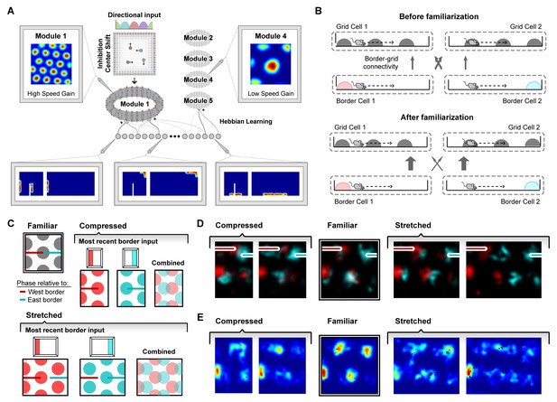
A model of border cell-grid cell interactions reproduces boundary-tethered shifts in grid phase during environmental deformations.
(A) The network model consisted of two layers: a border layer, where unit activity was determined by the presence of a boundary nearby (<12 cm) and in a particular allocentric direction, and a grid layer, where path integration implemented by a periodic attractor network of the form described in Burak and Fiete (2009) was used to generate five modules of grid units of different scales. During deformations, border fields scale in concert with changes to their preferred boundary and shift when their preferred boundary is displaced. (B) During familiarization, excitatory connections from border units to coactive grid units were strengthened at the expense of non-coactive connections. In deformed environments, border inputs reinstated the familiar phase relative to the most recently contacted boundary (schematically (C) and in the model (D)). (E) Averaged over time, these shifts in grid phase can resemble rescaling.
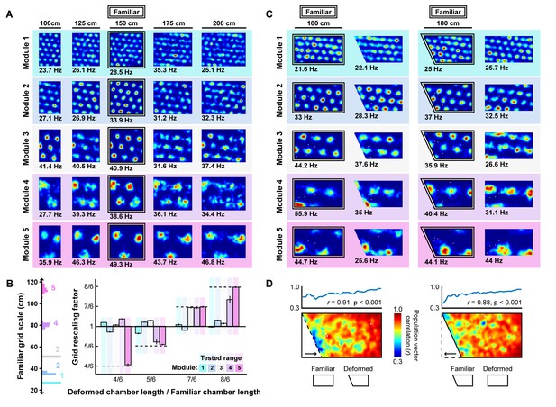
Grid unit responses to deformations of an open environment.
(A) Rate maps from one grid unit from each module across all rescaling deformations. Colors normalized to the maximum across each set of rate maps. Peak firing rate for each trial noted below the lower left corner of each map. (B) Grid rescaling factors for each module when the familiar open environment is rescaled to various chamber lengths (right). Error bars denote standard error of the mean (SEM) across 30 random grid units. Color denotes module. Distribution of grid scales for each module indicated (left). (C) Rate maps of one grid unit from each module across each partial deformation, plotted as in (A). (D) Correlation between the familiar and deformed environment rate maps across the population (150 grid units, 30 random cells from each module) at each location (bottom heatmaps) and averaged at each east-west position (top plots).
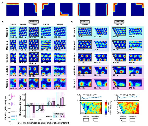
A rate-based network model with full-length border units reproduces boundary-tethered shifts, scale-dependent grid rescaling, and local distortions of the grid pattern during deformations.
The fields of border cells vary in coverage, with fields often covering the entire length of one wall. To ensure that our results were not exclusive to smaller field (50% the length of one border) border units, we reproduced our findings in a rate-based model in which all border units were active in fields 100% the length of one border. The following parameters were changed during rate-based model simulations: 64 border units were simulated; each grid module was composed of a 32 x 32 unit neural sheet; the grid translation scale factor ; the learning rate .= 0.000075; weight of grid unit radial uniform inhibition was set to -0.045. Stochastic spiking dynamics were eliminated and instead the output activation of each unit was determined by setting (A) Examples of rate-based border units. (B) Reproduction of scale-dependent grid rescaling (Figure 5A, B). (C) Reproduction of local distortion of the grid pattern during partial deformation (Figure 5C, D).
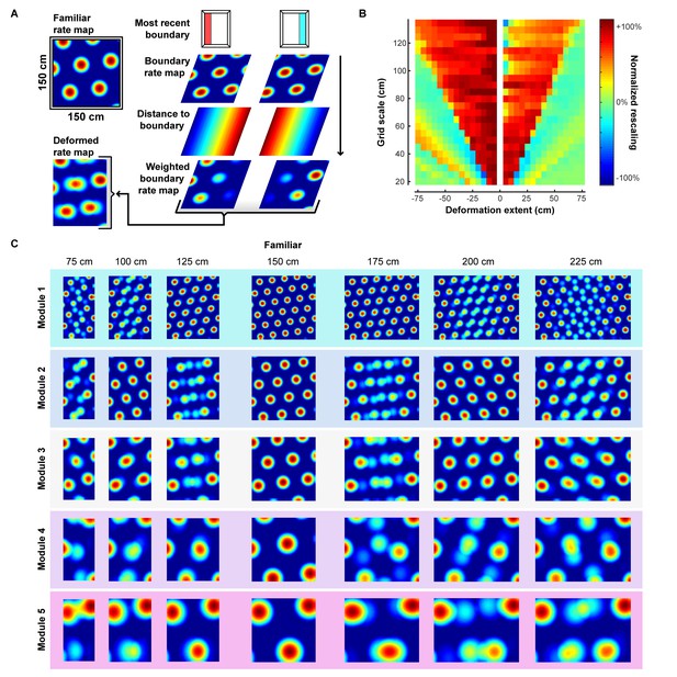
Scale-dependent rescaling arises from boundary-tethered shifts in simulations without plasticity.
In the main text, simulations were carried out over a limited range of grid scales and deformation extents because of computational constraints. (A) To extend this analysis to a much wider range of conditions, and to verify that our results are independent of the specific implementation of the model, we examined the effects of boundary-tethered grid shifts imposed directly on grid patterns. To do so, we first created familiar environment grid cell rate maps by overlapping and rectifying three 60°-offset sine waves (Bush et al., 2014). Next, we created predicted boundary rate maps as described in the main text (Figure 3—figure supplement 1), with sampling biases for each boundary rate map approximated as the inverse distance from the corresponding boundary. (B) Grid rescaling when a familiar 150 cm x 150 cm square environment is deformed as a function of grid scale and deformation extent. Grid rescaling normalized to range from no rescaling (0%) to a matched rescaling (100%). Note the dependence of the appearance of rescaling on grid scale and deformation extent, as well as the abrupt transition from the appearance of rescaling to a lack of an appearance of rescaling with more extreme deformations. (C) Example non-network simulated rate maps of various scales (30 cm, 45 cm, 60 cm, 90 cm, 120 cm) during a subset of deformations.
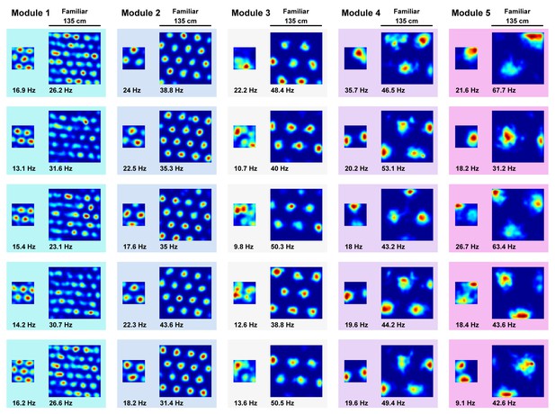
A more extreme compression deformation does not produce matched rescaling.
Although grid rescaling was reported during deformation in two electrophysiological studies (Barry et al., 2007; Stensola et al., 2012), another study implementing a more extreme compression deformation experiment did not observe a matched rescaling, that is a rescaling in which the deformed rate map resembled a compressed version of the familiar rate map, in grid cells (Savelli et al., 2008). To test whether the boundary-tethered model could account for a lack of rescaling during this more extreme compression, we familiarized the naive virtual rat with a 135 cm x 135 cm square environment. After this familiarization, the rat then again explored the familiar environment and a compressed 58 cm x 58 cm version of this environment without new learning. During this extreme compression, the grid patterns of modeled grid units did not resemble a matched rescaling of the familiar rate map, although distortions of the grid pattern were observed. Five random grid units from each module, peak firing rate denoted in bold below each map. Color normalized to the maximum for each rate map.
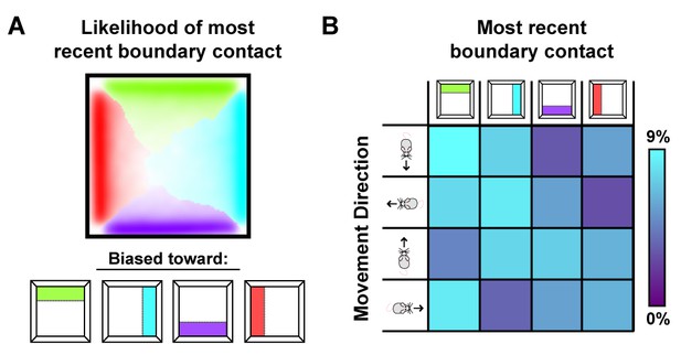
Sampling biases are correlated with the most recently contacted boundary.
(A) Likelihood of having most recently contacted each border as a function of location in a square environment. Hue indicates the most likely recently contacted boundary; saturation denotes the strength of the bias (white – 25% likelihood of sampling; fully saturated – 100% likelihood of sampling). Data from (Stensola et al., 2012). (B) Joint probability distribution depicting the relationship between movement direction and the most recently contacted boundary. Data from (Stensola et al., 2012).
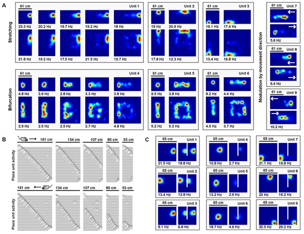
Place units learned from grid unit inputs reproduce heterogeneous place field distortions.
(A) Place unit rate maps when a familiar open environment is stretched. Place fields exhibit stretching, bifurcation, and emergent modulation by movement direction (indicated by white arrows). Colors normalized to the peak for each rate map. Peak firing rate noted below the lower left corner of each map. Note that peak firing rate tends to decrease with more extreme deformations for cells with place fields further from boundaries. (B) Place unit activity for all 64 place units during compressions of a familiar linear track, separated by (top) eastward and (bottom) westward laps. Each line indicates the firing rate of a single place unit at each location across the entire track during movement in the specified direction, normalized to the familiar track peak rate. Units sorted by place field location on the familiar track. Note that, during compressions, the place code unfolds as if anchored to the beginning of the track until the end of the track is encountered, at which point the familiar end-of-track place units are reactivated. (C) Place unit rate maps demonstrating a mix of place field (left) duplication, (middle) inhibition, and (right) perseverance when a new boundary (white line) is inserted in a familiar open environment. Colors normalized to the maximum of both rate maps. Peak firing rate noted below the lower left corner of each map.
Additional files
-
Transparent reporting form
- https://doi.org/10.7554/eLife.38169.020


