CaImAn an open source tool for scalable calcium imaging data analysis
- Flatiron Institute, Simons Foundation, United States
- Columbia University, United States
- ECE Paris, France
- University of California, Los Angeles, United States
- Princeton University, United States
- Cold Spring Harbor Laboratory, United States
Figures
Figure 1
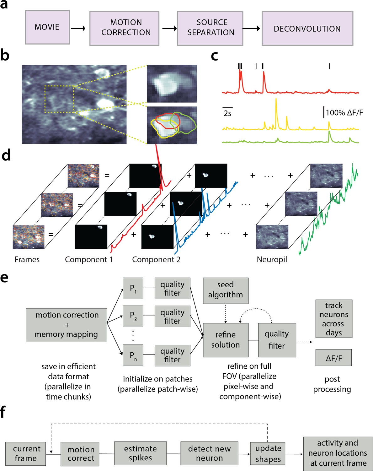
Processing pipeline of CaImAn for calcium imaging data.
(a) The typical pre-processing steps include (i) correction for motion artifacts, (ii) extraction of the spatial footprints and fluorescence traces of the imaged components, and (iii) deconvolution of the neural activity from the fluorescence traces. (b) Time average of 2000 frames from a two-photon microscopy dataset (left) and magnified illustration of three overlapping neurons (right), as detected by the CNMF algorithm. (c) Denoised temporal components of the three neurons in (b) as extracted by CNMF and matched by color (in relative fluorescence change, ). (d) Intuitive depiction of CNMF. The algorithm represents the movie as the sum of spatially localized rank-one spatio-temporal components capturing neurons and processes, plus additional non-sparse low-rank terms for the background fluorescence and neuropil activity. (e) Flow-chart of the CaImAn batch processing pipeline. From left to right: Motion correction and generation of a memory efficient data format. Initial estimate of somatic locations in parallel over FOV patches using CNMF. Refinement and merging of extracted components via seeded CNMF. Removal of low quality components. Final domain dependent processing stages. (f) Flow-chart of the CaImAn online algorithm. After a brief mini-batch initialization phase, each frame is processed in a streaming fashion as it becomes available. From left to right: Correction for motion artifacts. Estimation of activity from existing neurons, identification and incorporation of new neurons. The spatial footprints of inferred neurons are also updated periodically (dashed lines).
Figure 2
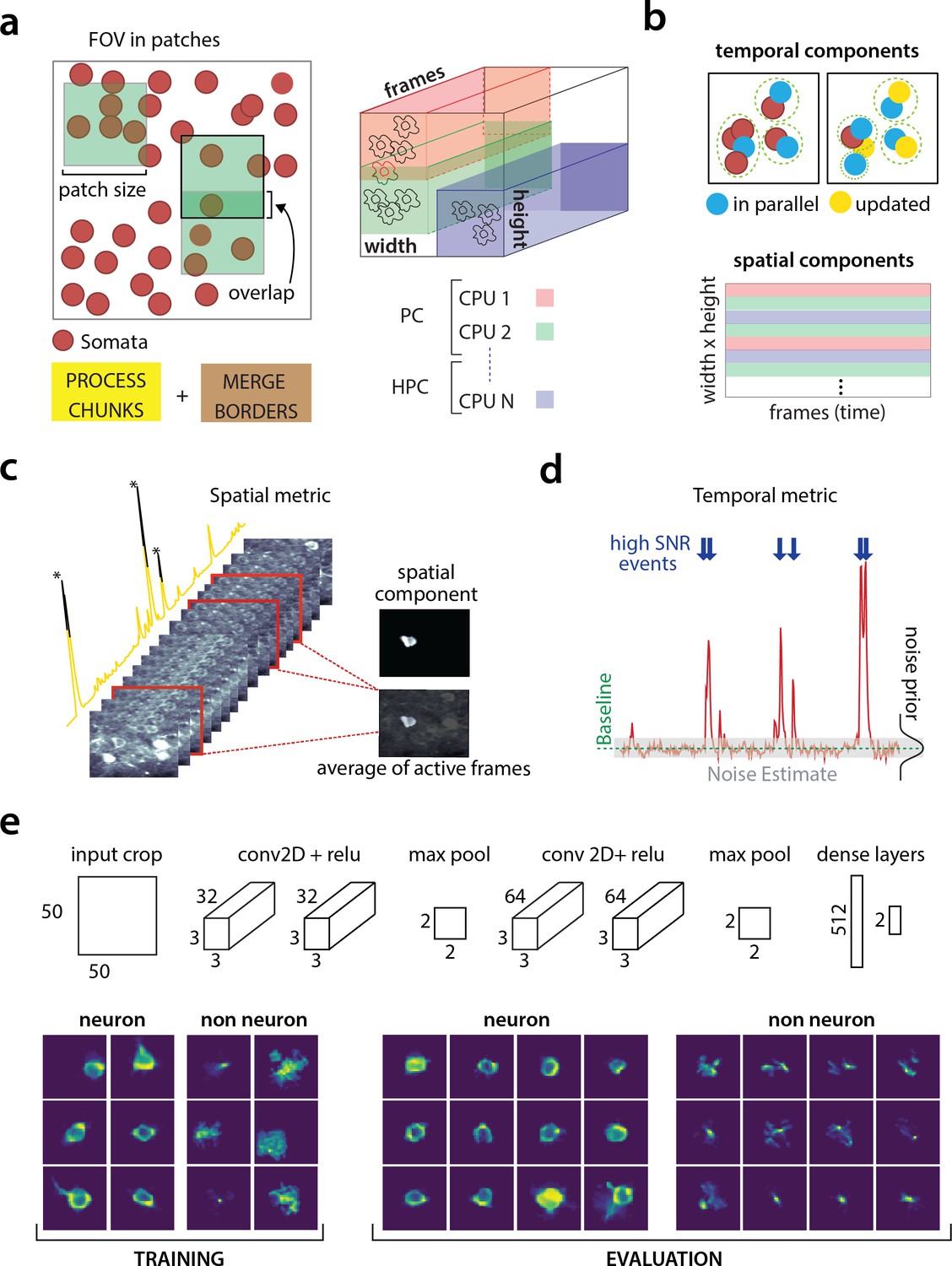
Parallelized processing and component quality assessment for CaImAn batch.
(a) Illustration of the parallelization approach used by CaImAn batch for source extraction. The data movie is partitioned into overlapping sub-tensors, each of which is processed in an embarrassingly parallel fashion using CNMF, either on local cores or across several machines in a HPC. The results are then combined. (b) Refinement after combining the results can also be parallelized both in space and in time. Temporal traces of spatially non-overlapping components can be updated in parallel (top) and the contribution of the spatial footprints for each pixel can be computed in parallel (bottom). Parallelization in combination with memory mapping enable large scale processing with moderate computing infrastructure. (c) Quality assessment in space: The spatial footprint of each real component is correlated with the data averaged over time, after removal of all other activity. (d) Quality assessment in time: A high SNR is typically maintained over the course of a calcium transient. (e) CNN based assessment. Top: A 4-layer CNN based classifier is used to classify the spatial footprint of each component into neurons or not, see Materials and methods (Classification through CNNs) for a description. Bottom: Positive and negative examples for the CNN classifier, during training (left) and evaluation (right) phase. The CNN classifier can accurately classify shapes and generalizes across datasets from different brain areas.
Figure 3 with 1 supplement
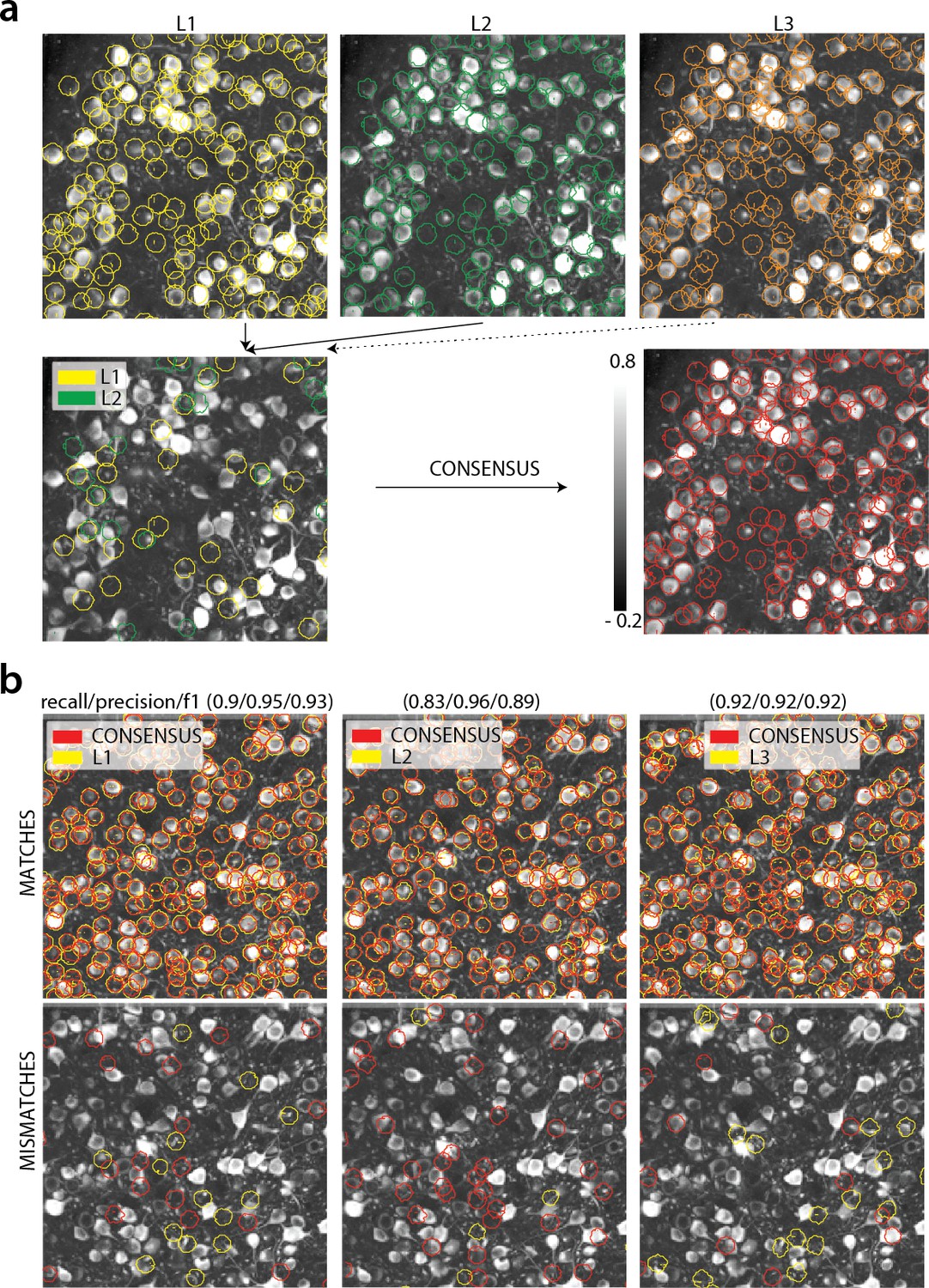
Consensus annotation generation.
(a) Top: Individual manual annotations on the dataset K53 (only part of the FOV is shown) for labelers L1 (left), L2 (middle), L3(right). Contour plots are plotted against the max-correlation image of the dataset. Bottom: Disagreements between L1 and L2 (left), and consensus labels (right). In this example, consensus considerably reduced the number of initially selected neurons. (b) Matches (top) and mismatches (bottom) between each individual labeler and consensus annotation. Red contours on the mismatches panels denote false negative contours, that is components in the consensus not selected by the corresponding labeler, whereas yellow contours indicate false positive contours. Performance of each labeler is given in terms of precision/recall and score and indicates an unexpected level of variability between individual labelers.
Figure 3—figure supplement 1
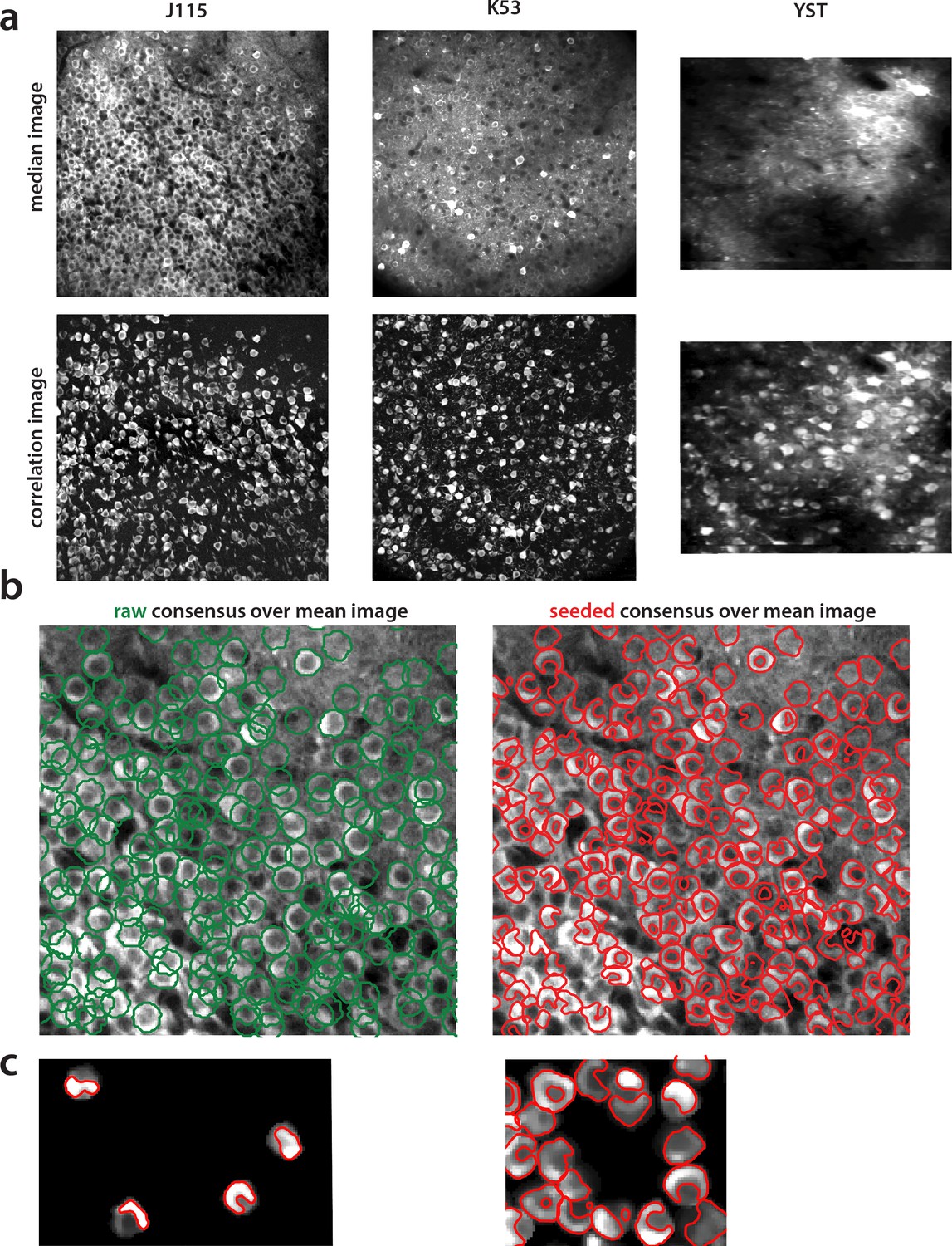
Construction of components obtained from consensus annotation.
(a) Correlation image can efficiently display active neurons. Comparison of median across time (top) and max-correlation (bottom) image for annotated datasets J115 (left), K53 (middle) and YST (right). In all cases, the correlation image aids in manual annotation by providing an efficient way to remove neuropil contamination and visualize the footprints of active neurons. (b) Contour plots of manual annotations (left) vs spatial footprints obtained after running SeededInitialization (right), for dataset J115 overlaid against the mean image. Manual annotations are restricted to be of ellipsoid shape whereas pre-processing with SeededInitialization allows the spatial footprints to adapt to the footprint of each neuron in the FOV. (c) Thresholding of spatial footprints selects the most prominent part of each neuron for comparison against ground truth. Left. Four examples of non thresholded components overlaid to their corresponding contours. Right. Same as left, but including all neurons within a small region. Finding an optimal threshold to generate consistent binary masks can be challenging.
Figure 4 with 2 supplements
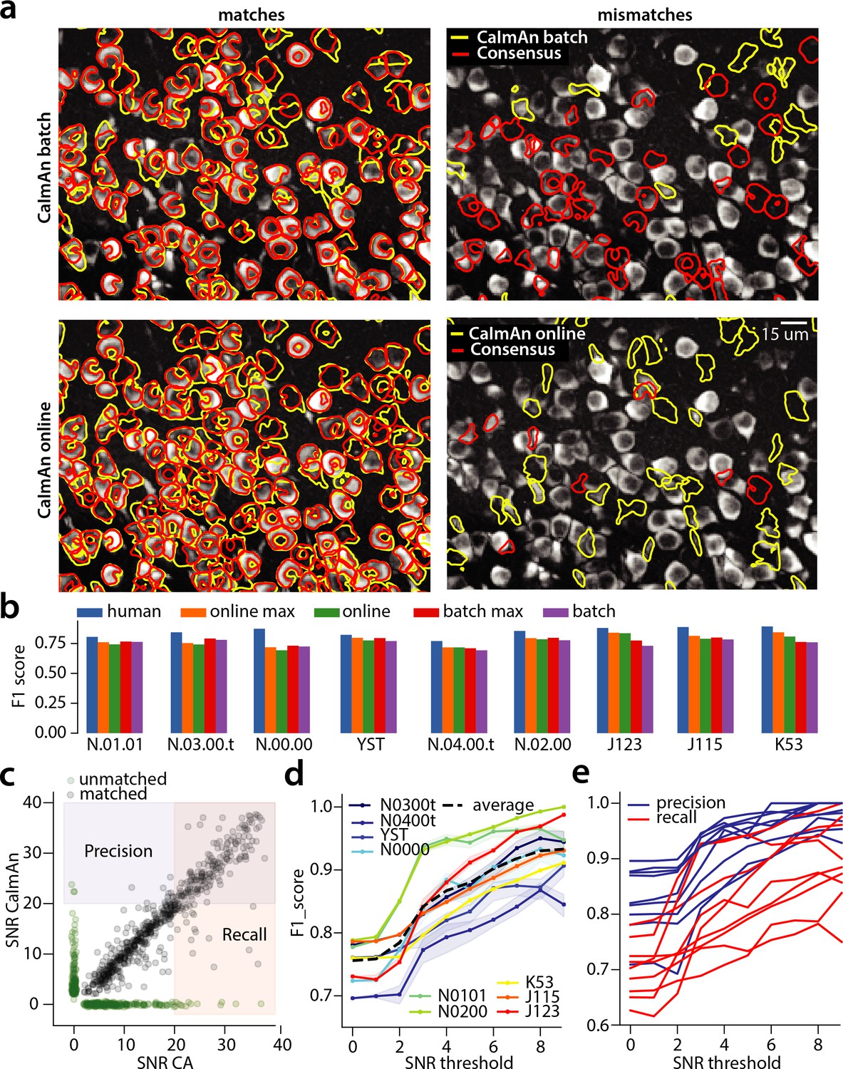
Evaluation of CaImAn performance against manually annotated data.
(a) Comparison of CaImAn batch (top) and CaImAn online (bottom) when benchmarked against consensus annotation for dataset K53. For a portion of the FOV, correlation image overlaid with matches (left panels, red: consensus, yellow: CaImAn) and mismatches (right panels, red: false negatives, yellow: false positives). (b) Performance of CaImAn batch, and CaImAn online vs average human performance (blue). For each algorithm the results with both the same parameters for each dataset and with the optimized per dataset parameters are shown. CaImAn batch and CaImAn online reach near-human accuracy for neuron detection. Complete results with precision and recall for each dataset are given in Table 1. (c–e) Performance of CaImAn batch increases with peak SNR. (c) Example of scatter plot between SNRs of matched traces between CaImAn batch and consensus annotation for dataset K53. False negative/positive pairs are plotted in green along the x- and y-axes respectively, perturbed as a point cloud to illustrate the density. Most false positive/negative predictions occur at low SNR values. Shaded areas represent thresholds above which components are considered for matching (blue for CaImAn batch and red for consensus selected components) (d) score and upper/lower bounds of CaImAn batch for all datasets as a function of various peak SNR thresholds. Performance of CaImAn batch increases significantly for neurons with high peak SNR traces (see text for definition of metrics and the bounds). (e) Precision and recall of CaImAn batch as a function of peak SNR for all datasets. The same trend is observed for both precision and recall.
Figure 4—figure supplement 1
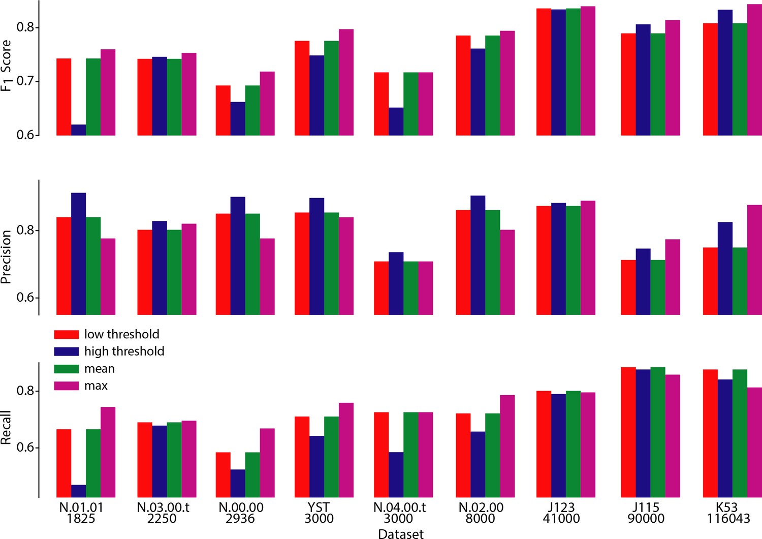
Performance of CaImAn online over different choices of parameters.
Performance of CaImAn online over different choices of three parameters: scores (top), Precision (middle) and Recall (bottom) are shown for all labeled datasets for four different cases: low threshold/large number setting (red) where , high threshold/low number setting where , and setting that maximizes performance averaged over all datasets (green) . The maximum score (and corresponding precision/recall) for each dataset is also shown (magenta). Lower threshold settings are more desirable for shorter datasets (N.03.00.t, N.04.00.t, N.00.00, N.01.01, YST) because they achieve high recall rates without a big penalty in precision. On the contrary, higher threshold settings are more desirable for longer datasets (J115, J123, K53) because they achieve high precision without a big penalty in recall.
Figure 4—figure supplement 2
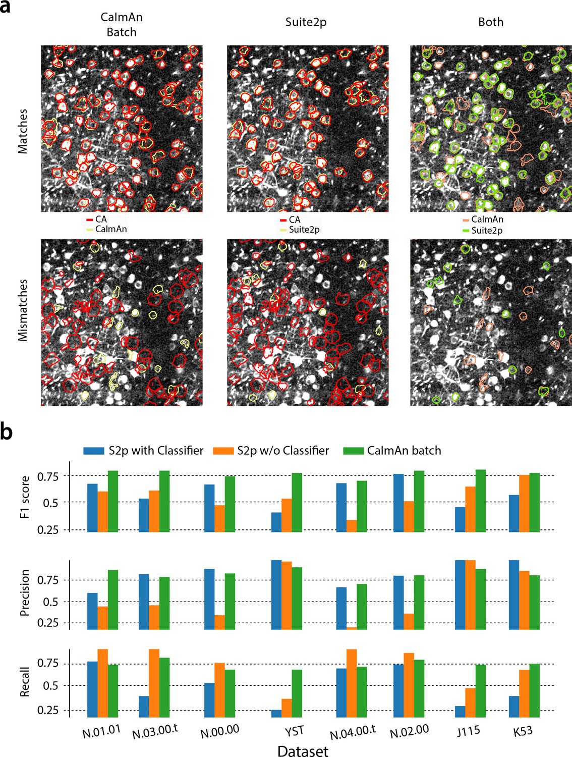
CaImAn batch outperforms the Suite2p algorithm in all datasets when benchmarked against the consensus annotation.
(a) Contour plots of selected components against consensus annotation (CA) for (left) and Suite2p with the use of a classifier (middle) and direct comparison between the algorithms (right) for the test dataset N.00.00. identifies better components with a weak footprint in the summary correlation image. (b) Performance metrics score (top), precision (middle) and recall (bottom), for Suite2p (with and the without the use of the classifier) and for the eight test datasets. consistently outperforms Suite2p, which can have significant variations between precision and recall. See Materials and methods (Comparison with Suite2p) for more details on the comparison.
Figure 5
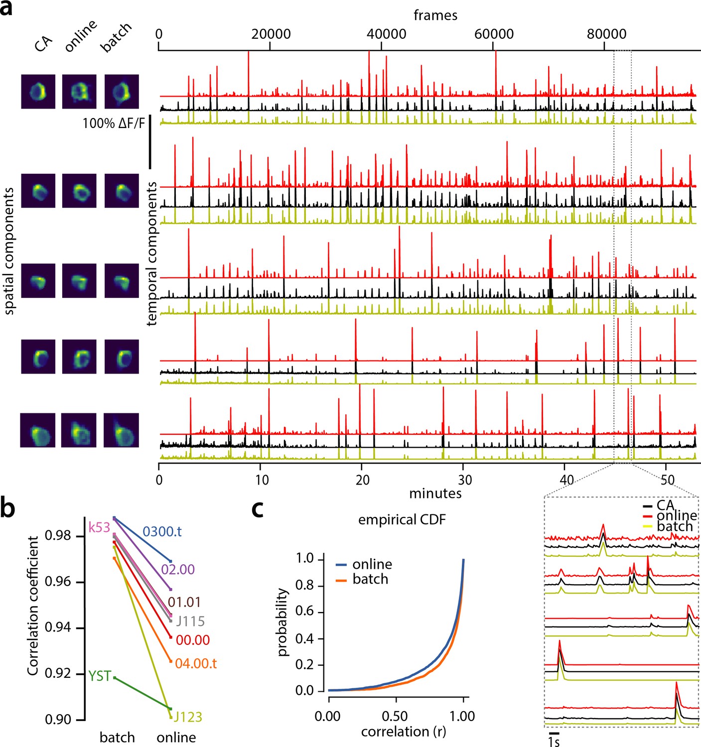
Evaluation of CaImAn extracted traces against traces derived from consensus annotation.
(a) Examples of shapes (left) and traces (right) are shown for five matched components extracted from dataset K53 for consensus annotation (CA, black), CaImAn batch (yellow) and CaImAn online (red) algorithms. The dashed gray portion of the traces is also shown magnified (bottom-right). Consensus spatial footprints and traces were obtained by seeding CaImAn with the consensus binary masks. The traces extracted from both versions of CaImAn match closely the consensus traces. (b) Slope graph for the average correlation coefficient for matches between consensus and CaImAn batch, and between consensus and CaImAn online. Batch processing produces traces that match more closely the traces extracted from the consensus labels. (c) Empirical cumulative distribution functions of correlation coefficients aggregated over all the tested datasets. Both distributions exhibit a sharp derivative close to 1 (last bin), with the batch approach giving better results.
Figure 6 with 2 supplements
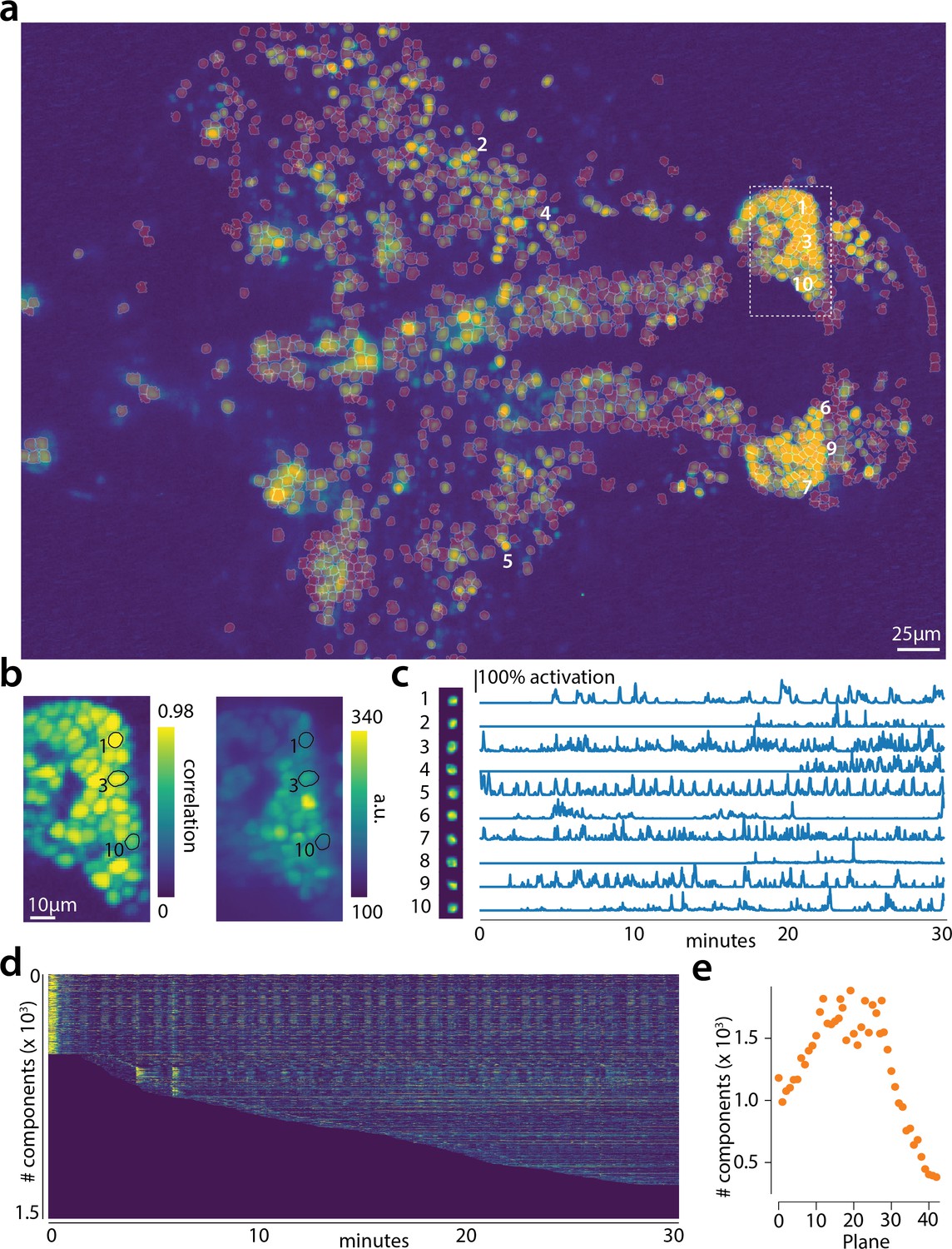
Online analysis of a 30 min long whole brain recording of the zebrafish brain.
(a) Correlation image overlaid with the spatial components (in red) found by the algorithm (portion of plane 11 out of 45 planes in total). (b) Correlation image (left) and mean image (right) for the dashed region in panel (a) with superimposed the contours of the neurons marked in (a). (c) Spatial (left) and temporal (right) components associated to the ten example neurons marked in panel (a). (d) Temporal traces for all the neurons found in the FOV in (a); the initialization on the first 200 frames contained 500 neurons (present since time 0). (e) Number of neurons found per plane (See also Figure 6—figure supplement 1 for a summary of the results from all planes).
Figure 6—figure supplement 1
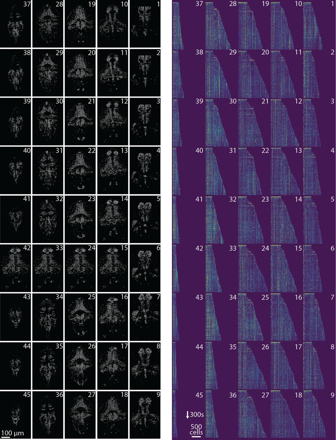
Spatial and temporal components for all planes.
Profile of spatial (left) and temporal (right) components found in each plane of the whole brain zebrafish recording. (Left) Components are extracted with CaImAn online and then max-thresholded. (Right) See Results section for a complete discussion. .
Figure 6—video 1
Results of CaImAn online initialized by CaImAn batch on a whole brain zebrafish dataset.
Each panel shows the active neurons in a given plane (top-to-bottom) without any background activity. See the text for more details.
Figure 7
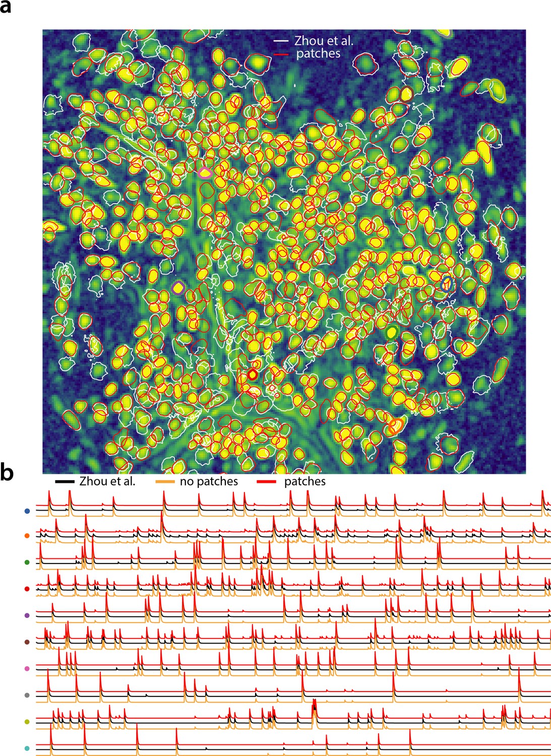
Analyzing microendoscopic 1 p data with the CNMF-E algorithm using CaImAn batch .
(a) Contour plots of all neurons detected by the CNMF-E (white) implementation of Zhou et al. (2018) and CaImAn batch (red) using patches. Colors match the example traces shown in (b), which illustrate the temporal components of 10 example neurons detected by both implementations CaImAn batch . reproduces with reasonable fidelity the results of Zhou et al. (2018).
Figure 8
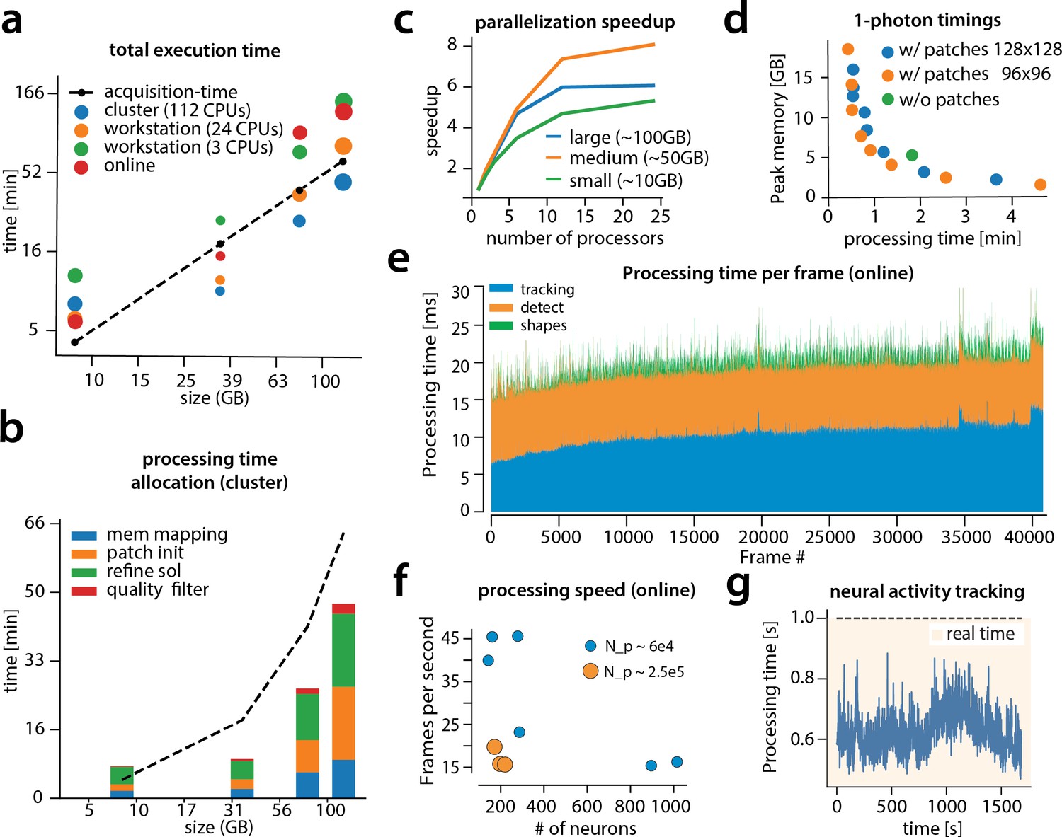
Time performance of CaImAn batch and CaImAn online for four of the analyzed datasets (small, medium, large and very large).
(a) Log-log plot of total processing time as a function of data size for CaImAn batch two-photon datasets using different processing infrastructures: (i) a desktop with three allocated CPUs (green), (ii) a desktop with 24 CPUs allocated (orange), and (iii) a HPC where 112 CPUs are allocated (blue). The results indicate a near linear scaling of the processing time with the size of dataset, with additional dependence on the number of found neurons (size of each point). Large datasets ( GB) can be seamlessly processed with moderately sized desktops or laptops, but access to a HPC enables processing with speeds faster than the acquisition time (considered 30 Hz for a 512512 FOV here). However, for smaller datasets the advantages of adopting a cluster vanishes, because of the inherent overhead. The results of CaImAn online using the laptop, using the ‘strict’ parameter setting (Figure 4—figure supplement 1), are also plotted in red indicating near real-time processing speed. (b) Break down of processing time for CaImAn batch (excluding motion correction). Processing with CNMF in patches and refinement takes most of the time for CaImAn batch. (c) Computational gains for CaImAn batch due to parallelization for three datasets with different sizes. The parallelization gains are computed by using the same 24 CPU workstation and utilizing a different number of CPUs for each run. The different parts of the algorithm exhibit the same qualitative characteristics (data not shown). (d) Cost analysis of CNMF-E implementation for processing a 6000 frames long 1p dataset. Processing in patches in parallel induces a time/memory tradeoff and can lead to speed gains (patch size in legend). (e) Computational cost per frame for analyzing dataset J123 with CaImAn onlne. Tracking existing activity and detecting new neurons are the most expensive steps, whereas udpating spatial footprints can be efficiently distributed among all frames. (f) Processing speed of CaImAn onlne for all annotated datasets. Overall speed depends on the number of detected neurons and the size of the FOV ( stands for number of pixels). Spatial downsampling can speed up processing. (g) Cost of neural activity online tracking for the whole brain zebrafish dataset (maximum time over all planes per volume). Tracking can be done in real-time using parallel processing.
Figure 9 with 1 supplement
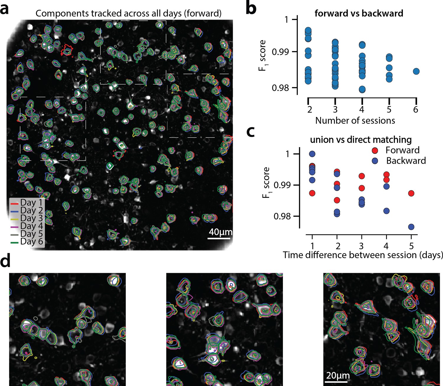
Components registered across six different sessions (days).
(a) Contour plots of neurons that were detected to be active in all six imaging sessions overlaid on the correlation image of the sixth imaging session. Each color corresponds to a different session. (b) Stability of multiday registration method. Comparisons of forward and backward registrations in terms of scores for all possible subsets of sessions. The comparisons agree to a very high level, indicating the stability of the proposed approach. (c) Comparison (in terms of score) of pair-wise alignments using readouts from the union vs direct alignment. The comparison is performed for both the forward and the backwards alignment. For all pairs of sessions the alignment using the proposed method gives very similar results compared to direct pairwise alignment. (d) Magnified version of the tracked neurons corresponding to the squares marked in panel (a). Neurons in different parts of the FOV exhibit different shift patterns over the course of multiple days, but can nevertheless be tracked accurately by the proposed multiday registration method.
Figure 9—figure supplement 1
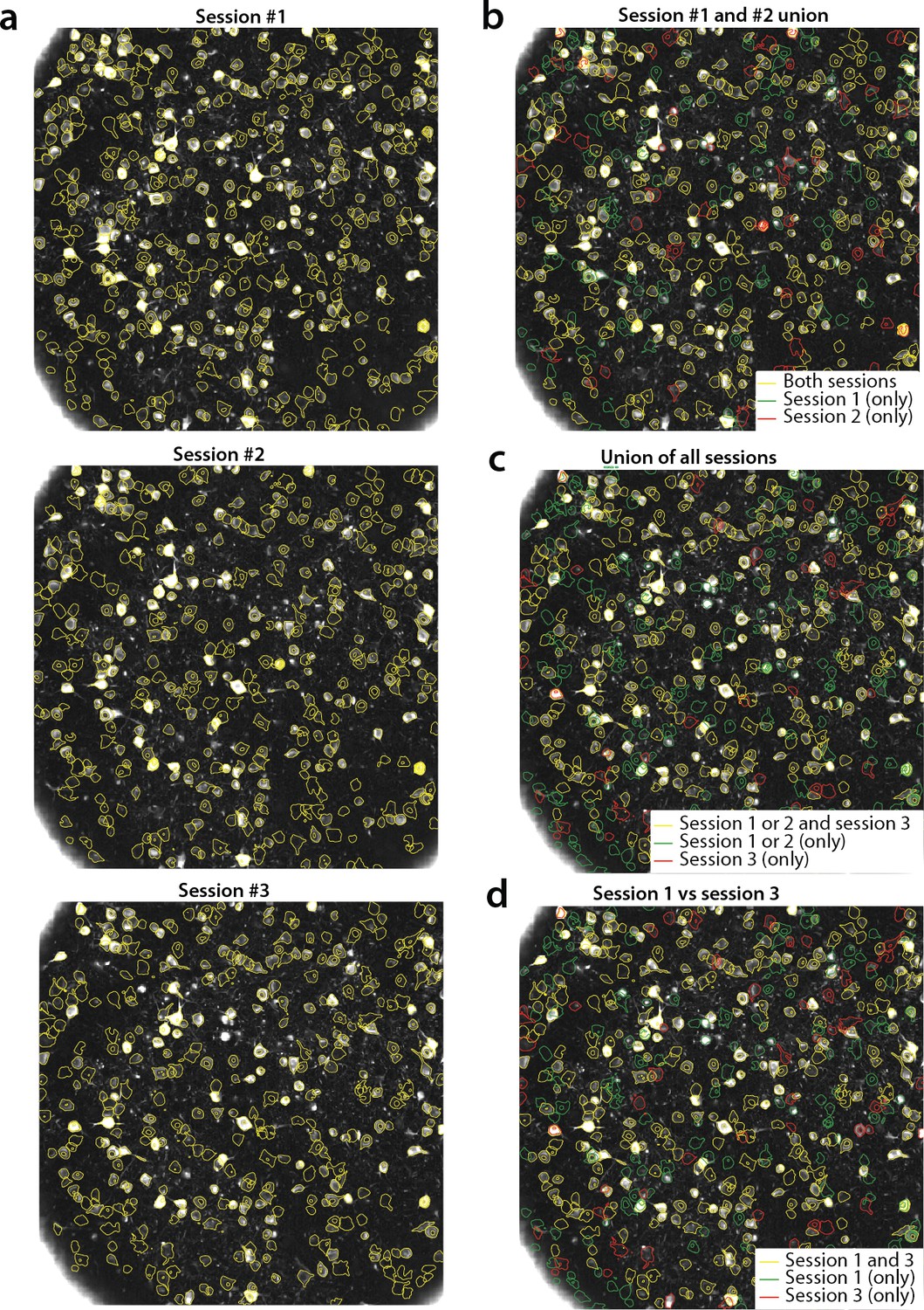
Tracking neurons across days; step-by-step description of multi session registration.
(a) Correlation image overlaid to contour plots of the neurons identified by in day 1 (top, 453 neurons), 2 (middle, 393 neurons) and 3 (bottom, 375 neurons). (b) Result of the pairwise registration between session 1 and 2. The union of distinct active components consists of the components that were active in i) both sessions (yellow - where only the components of session two are displayed), ii) only in session 2 (green), and iii) only in session 1 (red), aligned to the FOV of session 2. (c) At the next step the union of sessions 1 and 2 is registered with the results of session three to produce the union of all distinct components aligned to the FOV of session 3. (d) Registration of non-consecutive sessions (session 1 vs session 3) without pairwise registration. Keeping track of which session each component was active in enables efficient and stable comparisons.
Videos
Video 1
Depiction of CaImAn online on a small patch of in vivo cortex data.
Top left: Raw data. Bottom left: Footprints of identified components. Top right: Mean residual buffer and proposed regions for new components (in white squares). Enclosings of accepted regions are shown in magenta. Several regions are proposed multiple times before getting accepted. This is due to the strict behavior of the classifier to ensure a low number of false positives. Bottom right: Reconstructed activity.
Video 2
Depiction of CaImAn online on a single plane of mesoscope data courtesy of E. Froudarakis, J. Reimers and A. Tolias (Baylor College of Medicine).
Top left: Raw data. Top right: Inferred activity (without neuropil). Bottom left: Mean residual buffer and accepted regions for new components (magenta squares). Bottom right: Reconstructed activity.
Tables
Table 1
Results of each labeler, CaImAn batch and CaImAn online algorithms against consensus annotation.
Results are given in the form , and empty entries correspond to datasets not manually annotated by the specific labeler. The number of frames for each dataset, as well as the number of neurons that each labeler and algorithm found are also given. In italics the datasets used to train the CNN classifiers.
| Name # of frames | L1 | L2 | L3 | L4 | CaImAn batch | CaImAn online |
|---|---|---|---|---|---|---|
| N.01.01 1825 | 0.80 241(0.95, 0.69) | 0.89 287(0.96, 0.83) | 0.78 386(0.73, 0.84) | 0.75 289(0.80, 0.70) | 0.76 317(0.76, 0.77) | 0.75 298(0.81, 0.70) |
| N.03.00.t 2250 | X | 0.90 188(0.88, 0.92) | 0.85 215(0.78, 0.93) | 0.78 206(0.73, 0.83) | 0.78 154(0.76, 0.80) | 0.74 150(0.79, 0.70) |
| N.00.00 2936 | X | 0.92 425(0.93, 0.91) | 0.83 402(0.86, 0.80) | 0.87 358(0.96, 0.80) | 0.72 366(0.79, 0.67) | 0.69 259(0.87, 0.58) |
| YST 3000 | 0.78 431(0.76, 0.81) | 0.90 465(0.85, 0.97) | 0.82 505(0.75, 0.92) | 0.79 285(0.96, 0.67) | 0.77 332(0.85, 0.70) | 0.77 330(0.84, 0.70) |
| N.04.00.t 3000 | X | 0.69 471(0.54, 0.97) | 0.75 411(0.61, 0.97) | 0.87 326(0.78, 0.98) | 0.69 218(0.69, 0.70) | 0.7 260(0.68, 0.72) |
| N.02.00 8000 | 0.89 430(0.86, 0.93) | 0.87 382(0.88, 0.85) | 0.84 332(0.92, 0.77) | 0.82 278(1.00, 0.70) | 0.78 351(0.78, 0.78) | 0.78 334(0.85, 0.73) |
| J123 41000 | X | 0.83 241(0.73, 0.96) | 0.90 181(0.91, 0.90) | 0.91 177(0.92, 0.89) | 0.73 157(0.88, 0.63) | 0.82 172(0.85, 0.80) |
| J115 90000 | 0.85 708(0.96, 0.76) | 0.93 869(0.94, 0.91) | 0.94 880(0.95, 0.93) | 0.83 635(1.00, 0.71) | 0.78 738(0.87, 0.71) | 0.79 1091(0.71, 0.89) |
| K53 116043 | 0.89 795(0.96, 0.83) | 0.92 928(0.92, 0.92) | 0.93 875(0.95, 0.91) | 0.83 664(1.00, 0.72) | 0.76 809(0.80, 0.72) | 0.81 1025(0.77, 0.87) |
| mean ± std | 0.84±0.05(0.9±0.08, 0.8±0.08) | 0.87±0.07(0.85±0.13, 0.92±0.05) | 0.85±0.06(0.83±0.11, 0.88±0.06) | 0.83±0.09(0.91±0.1, 0.78±0.1) | 0.754±0.03(0.8±0.06, 0.72±0.05) | 0.762±0.05(0.82±0.06, 0.73±0.1) |
Table 2
Properties of manually annotated datasets.
For each dataset the duration, imaging rate and calcium indicator are given, as well as the number of active neurons selected after consensus between the manual annotators.
| Name | Area brain | Lab | Rate (Hz) | Size (TXY) | Indicator | Labelers | Neurons CA |
|---|---|---|---|---|---|---|---|
| NF.01.01 | Visual Cortex | Hausser | 7 | 1825 × 512 × 512 | GCaMP6s | 4 | 333 |
| NF.03.00.t | Hippocampus | Losonczy | 7 | 2250 × 498 × 467 | GCaMP6f | 3 | 178 |
| NF.00.00 | Cortex | Svoboda | 7 | 2936 × 512 × 512 | GCaMP6s | 3 | 425 |
| YST | Visual Cortex | Yuste | 10 | 3000 × 200 × 256 | GCaMP3 | 4 | 405 |
| NF.04.00.t | Cortex | Harvey | 7 | 3000 × 512 × 512 | GCaMP6s | 3 | 257 |
| NF.02.00 | Cortex | Svoboda | 30 | 8000 × 512 × 512 | GCaMP6s | 4 | 394 |
| J123 | Hippocampus | Tank | 30 | 41000 × 458 × 477 | GCaMP5 | 3 | 183 |
| J115 | Hippocampus | Tank | 30 | 90000 × 463 × 472 | GCaMP5 | 4 | 891 |
| K53 | Parietal Cortex | Tank | 30 | 116043 × 512 × 512 | GCaMP6f | 4 | 920 |
Table 3
Cross-validated results of each labeler, where each labeler’s performance is compared against the annotations of the rest of the labelers using a majority vote.
Results are given in the form score (precision, recall), and empty entries correspond to datasets not manually annotated by the specific labeler. The results indicate decreased performance compared to the consensus annotation annotations.
| Name | L1 | L2 | L3 | L4 | Mean |
|---|---|---|---|---|---|
| N.01.01 | 0.75 (0.73, 0.77) | 0.70 (0.58, 0.88) | 0.86 (0.81, 0.90) | 0.84 (0.92, 0.77) | 0.79 (0.76, 0.83) |
| N.03.00.t | X | 0.75 (0.69, 0.82) | 0.79 (0.67, 0.97) | 0.85 (0.76,0.97) | 0.8 (0.71,0.92) |
| N.00.00 | X | 0.87 (0.84,0.90) | 0.82 (0.75,0.91) | 0.72 (0.71,0.97) | 0.83 (0.76,0.93) |
| YST | 0.7 (0.93,0.56) | 0.79 (0.7,0.9) | 0.81 (0.76,0.86) | 0.77 (0.75,0.78) | 0.77 (0.78,0.78) |
| N.04.00.t | X | 0.79 (0.76,0.83) | 0.72 (0.60,0.89) | 0.68 (0.53,0.96) | 0.73 (0.63,0.89) |
| N.02.00 | 0.84 (0.97,0.75) | 0.88 (0.89,0.87) | 0.86 (0.79,0.94) | 0.81 (0.7,0.95) | 0.85 (0.83,0.88) |
| J123 | X | 0.9 (0.86,0.93) | 0.89 (0.84,0.93) | 0.77 (0.63,0.96) | 0.87 (0.88,0.88) |
| J115 | 0.85 (0.98,0.76) | 0.87 (0.80,0.97) | 0.88 (0.80,0.97) | 0.87 (0.93,0.82) | 0.85 (0.78,0.94) |
| K53 | 0.86 (0.98,0.77) | 0.9 (0.85,0.96) | 0.88 (0.8,0.96) | 0.89 (0.9,0.88) | 0.88 (0.88,0.89) |
| mean std | 0.8±0.06 (0.92±0.09,0.72±0.08) | 0.83±0.07 (0.77±0.1,0.9±0.05) | 0.83±0.05 (0.76±0.07,0.92±0.04) | 0.81±0.06 (0.76±0.13,0.9±0.08) | 0.82±0.06 (0.77±0.12,0889±0.06) |
Additional files
-
Transparent reporting form
- https://doi.org/10.7554/eLife.38173.031
Download links
A two-part list of links to download the article, or parts of the article, in various formats.
Downloads (link to download the article as PDF)
Open citations (links to open the citations from this article in various online reference manager services)
Cite this article (links to download the citations from this article in formats compatible with various reference manager tools)
CaImAn an open source tool for scalable calcium imaging data analysis
eLife 8:e38173.
https://doi.org/10.7554/eLife.38173


