Research Article

Physics of Living Systems

Body size-dependent energy storage causes Kleiber’s law scaling of the metabolic rate in planarians

Max Planck Institute of Molecular Cell Biology and Genetics, Germany
Max Planck Institute for the Physics of Complex Systems, Germany
FOM Institute AMOLF, The Netherlands
Helmholtz-Zentrum Dresden-Rossendorf, Institute of Resource Ecology, Germany
Massachusetts Institute of Technology, United States
Technische Universität Dresden, Germany

Jan 4, 2019

https://doi.org/10.7554/eLife.38187

Open access
Copyright information

Figures
Tables
Additional files

5 figures, 1 table and 2 additional files

Figures

Figure 1 with 1 supplement

Download asset Open asset

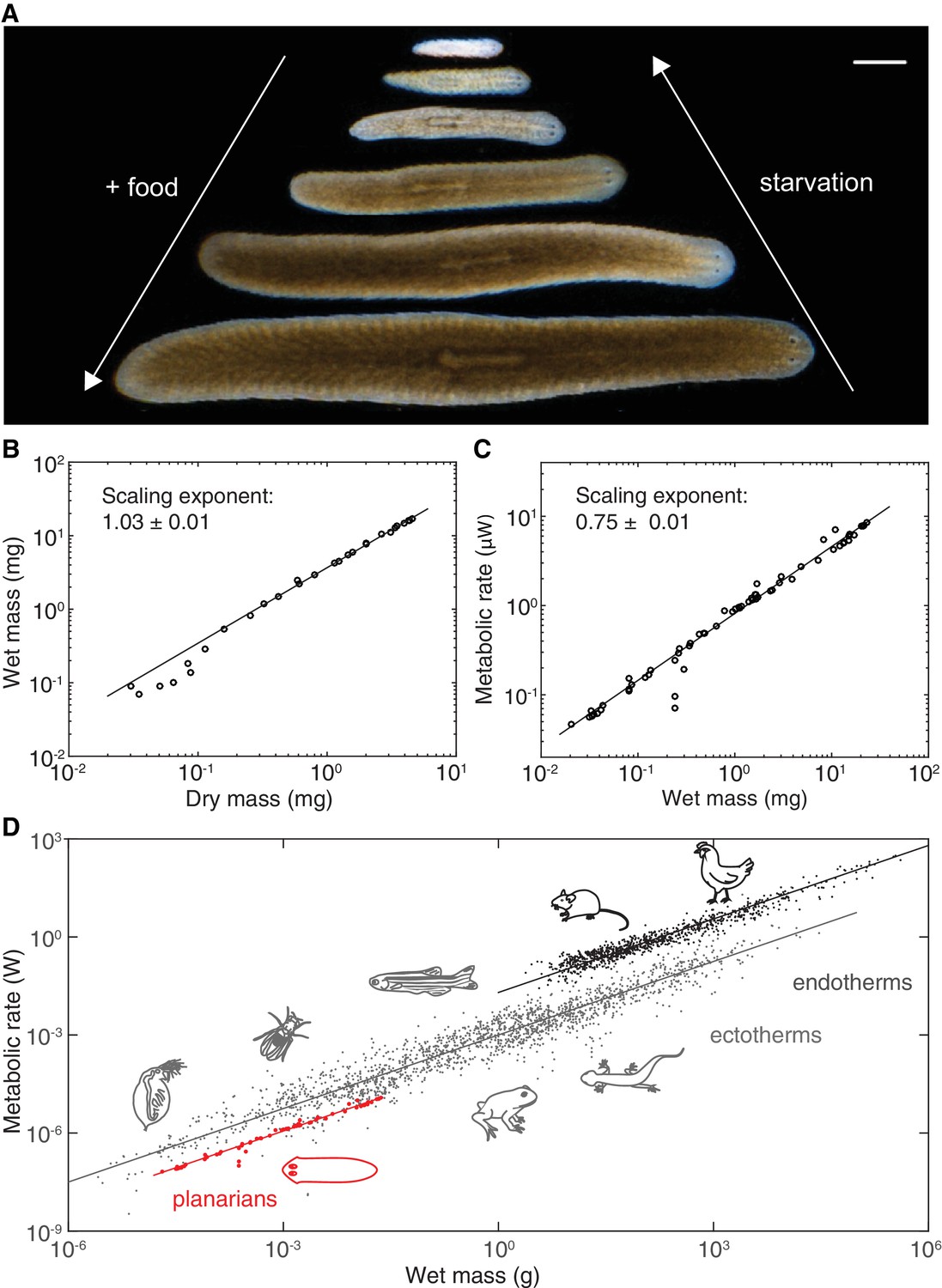
Kleiber’s law scaling during *S.mediterranea* body size changes.

(A) Feeding (growth) and starvation (degrowth) dependent body size changes of *Schmidtea mediterranea*. Scale bar, 1 mm. (B) Wet versus dry mass scaling with body size. The scaling exponent ± standard error was derived from a linear fit for wet mass > 0.5 mg and represents the exponent b of the power law *y = ax^b*. See Figure 1—source data 1 for numerical data. (C) Metabolic rate versus wet mass scaling by microcalorimetry. The metabolic rate was determined by a horizontal line fitted to the stabilised post-equilibration heat flow trace (Figure 1—figure supplement 1) and the post-experimental dry mass determination of all animals in the vial was re-converted into wet mass by the scaling relation from (B). Each data point represents a vial average of a size-matched cohort. The scaling exponent ± standard error was derived from a linear fit and represents the exponent b of the power law *y = ax^b*. (D) Metabolic rate versus wet mass scaling in planarians from (C) (red) in comparison with published interspecies comparisons (Makarieva et al., 2008) amongst ectotherms (grey) or endotherms (black). Dots correspond to individual measurements; black and blue solid lines trace the 3/4 scaling exponent; red line, linear fit to the planarian data. By convention (Makarieva et al., 2008), measurements from homeotherms obtained at different temperatures were converted to 37 °C, measurements from poikilotherms and our planarian measurements to 25 °C, using the following factor: $2^{(25^{\circ} C - 20^{\circ} C) / 10^{\circ} C} = 2^{0.5}$ (20 °C: planarian data acquisition temperature).

https://doi.org/10.7554/eLife.38187.002

Figure 1—source data 1 Numerical data wet mass vs. dry mass measurements.: https://doi.org/10.7554/eLife.38187.005
Download elife-38187-fig1-data1-v1.xlsx

Figure 1—figure supplement 1

Download asset Open asset

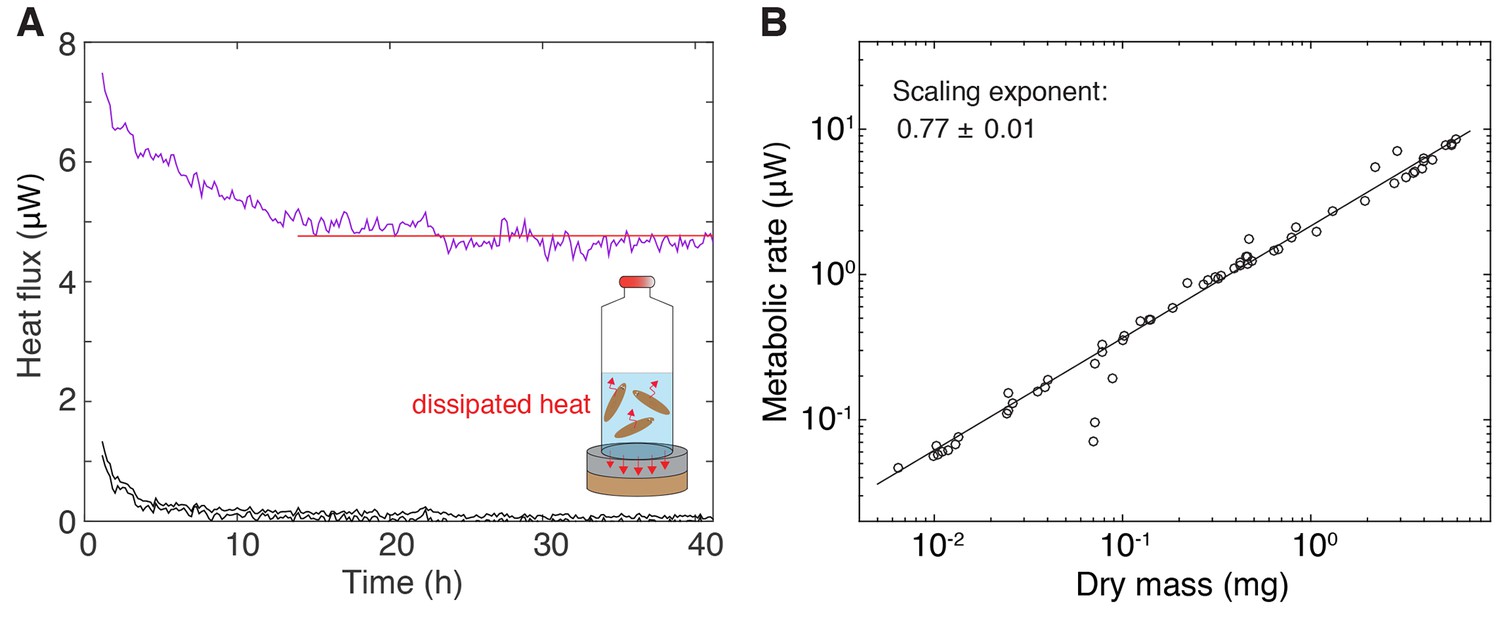
Measurement of metabolic rate.

(A) Inset: Cartoon representation of the experimental setup, comprising the enclosure of a cohort of size-matched test subjects into a vial and quantification of the heat flux via a thermoelectric detector. The shown traces are representative examples of heat flux over time measurements from a vial with animals (purple, top) or two controls without animals (black, bottom). The average metabolic rate was determined by manually fitting a horizontal line (red) through the stable section of the trace post the initial equilibration phase (evident initial signal relaxation in all traces during the first ~10 h). 21 out of 83 samples were excluded as no fit could be obtained due to high signal fluctuations. (B) Metabolic rate versus dry mass scaling in *S. mediterranea*. Circles represent individual metabolic rate measurements determined as described in A). Immediately after the end of the experiment, animals were recovered from the vial, dried and weighted. The plotted values represent metabolic rate and dry mass per animal, as obtained by dividing the total metabolic rate or total dry mass measurement by the number of size-matched animals within the cohort. The scaling exponent ± standard error was derived from a linear fit and represents the exponent b of the power law *y = ax^b*. See Figure 1—figure supplement 1—source data 1 for numerical data.

https://doi.org/10.7554/eLife.38187.003

Figure 1—figure supplement 1—source data 1 Raw data metabolic rate measurements.: https://doi.org/10.7554/eLife.38187.004
Download elife-38187-fig1-figsupp1-data1-v1.xlsx

Figure 2 with 3 supplements

Download asset Open asset

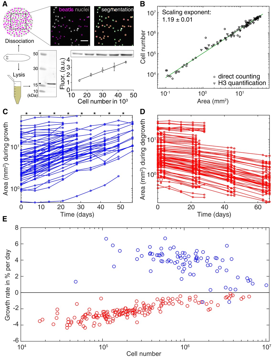
Growth and degrowth dynamics in *S.mediterranea*.

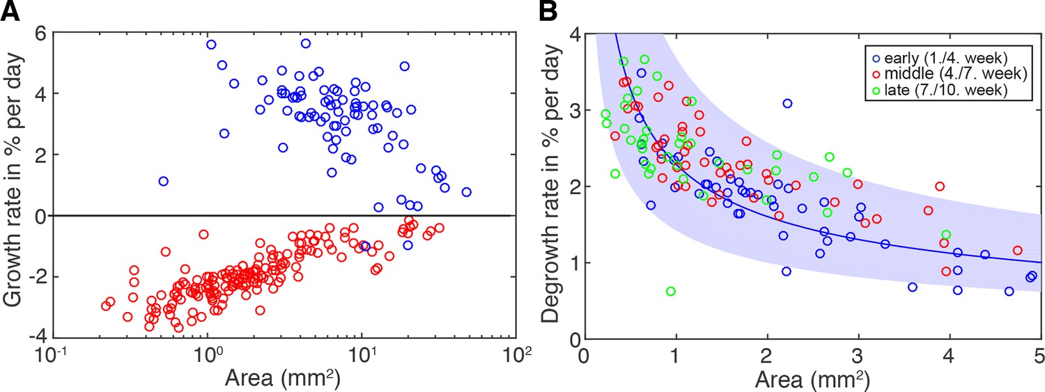
(A) Assays to measure organismal cell numbers. (Top) image-based quantification of nuclei (grey) versus tracer beads (magenta) following whole animal dissociation in presence of the volume tracer beads. (Bottom) Histone H3 protein quantification by quantitative Western blotting, which scales linearly with the number of FACS-sorted cells (bottom right). The line represents a fitted linear regression (data of 4 technical replicates) and serves as standard for converting the H3 band in planarian lysates (bottom left) run on the same gel into cell numbers. Values are shown as mean ± standard deviation. (B) Organismal cell number versus plan area scaling, by nuclei counts (circles) or Histone H3 protein amounts (triangles) (see also Figure 2—figure supplements 1 and 2). The scaling exponent ± standard error was derived from a linear fit and represents the exponent b of the power law *y = ax^b*. Each data point represents one individual animal and the mean of several technical replicates, Histone H3 method: nine independent experiments including five animals each; image-based approach: four independent experiments including 18, 10, 10 and 12 animals each. See Figure 2—source datas 1–3 for numerical data. (C) Plan area changes of individual animals during growth. * indicate feeding time points (1x per week). (D) Plan area change of individual animals during degrowth. (E) Size-dependence of growth (blue) and degrowth rates (red) (see also Figure 2—figure supplement 3A). Individual data points were calculated by exponential fits to traces in (C) and (D) (growth: two overlapping time windows, degrowth: three overlapping time windows) and using the cell number/area scaling law from (B) to express rates as % change in cell number/day. The positive growth rates and negative degrowth rates are plotted on the same axis to facilitate comparison of size dependence. See Figure 2—source data 5 for data of (C) and (D).

https://doi.org/10.7554/eLife.38187.006

Figure 2—source data 1 Numerical data cell number measurements.: https://doi.org/10.7554/eLife.38187.012
Download elife-38187-fig2-data1-v1.xlsx
Figure 2—source data 2 Raw numerical data Histone H3 method (quantitative Western blotting).: https://doi.org/10.7554/eLife.38187.013
Download elife-38187-fig2-data2-v1.xlsx
Figure 2—source data 3 CellProfiler results tables image-based approach.: https://doi.org/10.7554/eLife.38187.014
Download elife-38187-fig2-data3-v1.zip
Figure 2—source data 4 MATLAB code for extraction of planarian body size.: https://doi.org/10.7554/eLife.38187.015
Download elife-38187-fig2-data4-v1.zip
Figure 2—source data 5 Numerical data growth/degrowth.: https://doi.org/10.7554/eLife.38187.016
Download elife-38187-fig2-data5-v1.xlsx

Figure 2—figure supplement 1

Download asset Open asset

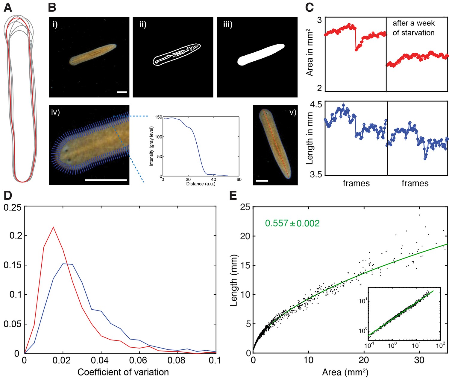
Measurement of planarian body size.

(A) Body outline variations of one individual extracted from multiple frames of a single movie. The red outline marks the outline in the first frame. (B) Illustration of the pipeline for extracting plan area and length measurements of individual planarians from movie sequences, see also (Werner et al., 2014). (i) raw movie frame, ii) use of a Canny filter on background-corrected frames to identify edges, iii) dilation-erosion cycle to fill segmentation gaps in a subsequent step, iv) refinement of animal perimeter by finding the steepest intensity change across the body edge (blue lines intersecting on the left, example plot of the intensity change across one blue line on the right), (v) resulting boundary outline (blue; yielding plan area measurement) and midline (red; yielding length measurement), overlaid on the original image to illustrate accuracy of the procedure. Stated plan area and length measurements in this manuscript always represent the median of up to 180 individually quantified movie frames displaying the same animal in an extended body posture. Scale bars, 1 mm. See Figure 2—source data 4 for MATLAB script. (C) Accuracy comparison between area (top, red) and length measurement traces (bottom, blue). The traces represent a concatenation of 2 independent movie sequences of the same animal, before (left half) and after 1 week of starvation (right half). The plan area trace illustrates better resolution of the degrowth during the starvation period, which is harder to discern in the noisier length measurements. (D) Histogram analysis of the coefficients of variation (ratio standard deviation/mean) across a data set of 2470 individual length versus plan area measurements determined as described in (**A–C**). The slight right shift of the length measurement histogram (blue) as compared to the area measurement histogram (red) quantitatively confirms the lower variability of the plan area measurements, which is why plan area was generally used as a size measure in this study. (E) Plot of the length versus plan area measurements as described in (**A–C**) of 1390 individual measurements selected to collectively represent the entire range of body sizes in *S. mediterranea*. Individual data points are represented by black dots, the green line represents a linear fit to the data in the log-log plot (inset). The tight fit over the entire size range demonstrates a tight regulation of body shape during growth/degrowth. The scaling exponent ± error was derived from the linear fit and represents the exponent b of the power law *y = ax^b*. See Figure 2—figure supplement 1—source data 1for data of (D) and (E).

https://doi.org/10.7554/eLife.38187.007

Figure 2—figure supplement 1—source data 1 Numerical data for Figure 2—figure supplement 1D and E.: https://doi.org/10.7554/eLife.38187.008
Download elife-38187-fig2-figsupp1-data1-v1.xlsx

Figure 2—figure supplement 2

Download asset Open asset

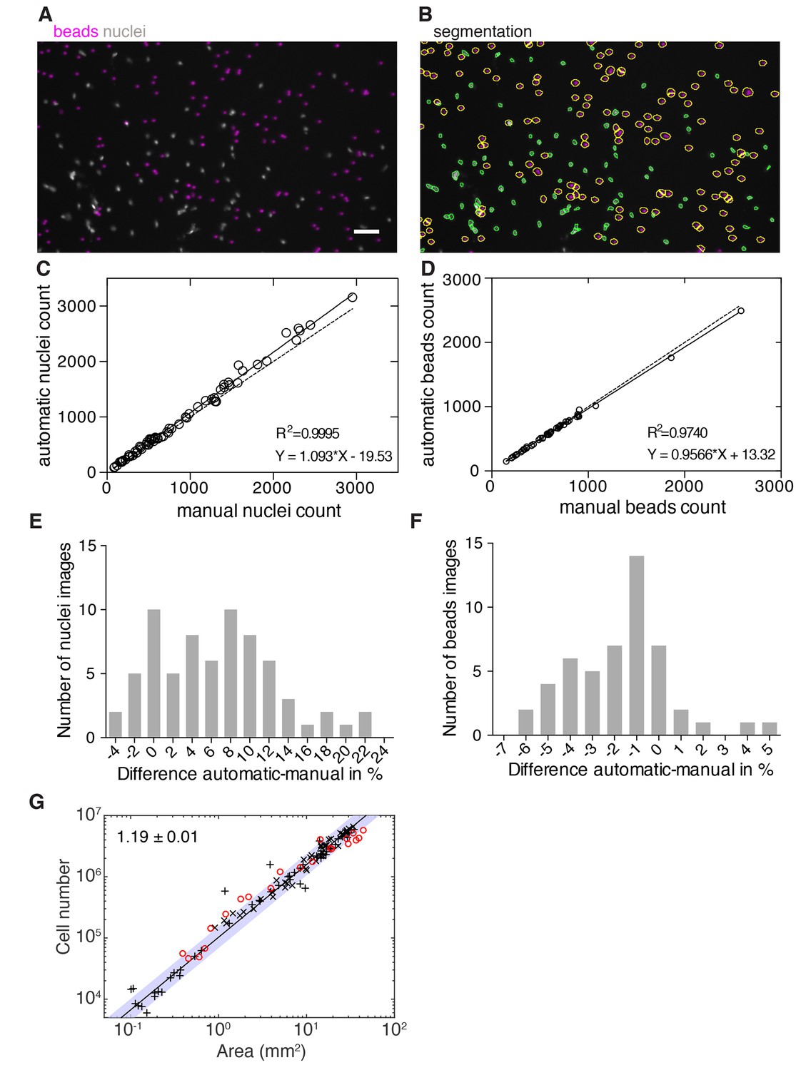
Validation of image-based quantification of organismal cell number.

(A) Representative image of a whole animal macerate spotted on imaging plates and imaged with an automated microscope (see methods). Stained nuclei are shown in grey and added volume tracer beads in magenta. Scale bar, 25 µm. (B) Automatic segmentation of nuclei (green contours) and beads (yellow contours) in the same image as shown in (A). (C) Automatic versus manual nuclei counts in a subset of images used in Figure 2B (69 images from three experiments were manually annotated and analysed). The high correlation confirms the accuracy of the nuclear counts under experimental conditions. Solid line, linear regression; dotted line, hypothetical perfect match between automatic and manual counts (*y = x*). (D) Automatic versus manual bead counts on a subset of images used in Figure 2B (50 images from three experiments were manually annotated and analysed). The value of the correlation coefficient confirms the accuracy of the bead counts under experimental conditions. Solid line, linear regression; dotted line, hypothetical perfect match between automatic and manual counts (*y = x*). (E) Histogram showing the (binned) number of measured differences per image between the automatic and manual nuclei counts shown in (C). (F) Histogram showing the number of (binned) measured differences per image between the automatic and manual bead counts shown in (D). See Figure 2—figure supplement 2—source data 1for raw and numerical data of (C)-(F) as well as the image analysis pipeline built in CellProfiler. (G) Organismal cell number versus area scaling of 3 weeks starved animals (red circles, one experiment) in comparison with the organismal cell number versus plan area scaling of 1–2 weeks starved animals as shown in Figure 2B (black crosses). The overlap of both data sets indicates no long-term effect of feeding history on the cell number-area scaling relationship. The scaling exponent ± standard error was derived from a linear fit to the black crosses (1–2 weeks starved) and represents the exponent b of the power law *y = ax^b*. The blue band indicates the 95% confidence interval of the fit. See Figure 2—source data 1 for numerical data.

https://doi.org/10.7554/eLife.38187.009

Figure 2—figure supplement 2—source data 1 CellProfiler pipeline, numerical data, raw images and segmentation for validation of image-based cell counting.: https://doi.org/10.7554/eLife.38187.010
Download elife-38187-fig2-figsupp2-data1-v1.zip

Figure 2—figure supplement 3

Download asset Open asset

Degrowth rates are independent of feeding history.

(A) Growth (blue) and degrowth rates (red) plotted as the % change in area/day. Individual data points were calculated by exponential fits to individual animal growth/degrowth trajectories shown in Figure 2C and D (growth: two overlapping time windows, degrowth three overlapping time windows). The positive growth rates and negative degrowth rates are plotted on the same axis to facilitate comparison of size dependencies. These data were also used to generate Figure 2E by conversion into % change in cell number/day using the cell number/area scaling relationship from Figure 2B. (B) Degrowth rates from (A) colour-coded according to time since start of food deprivation; early (blue), 1–4 weeks; middle (red), 4–7 weeks; late (green), 7–10 weeks. Solid line represents a power law (*y = ax^b*) fit to the early (blue) time points. Blue band represents the 95% confidence interval for the early (blue) degrowth rates; note that middle (red) and late (green) degrowth rates lie mostly within this interval, indicating the lack of a feeding history dependence within the covered time interval.

https://doi.org/10.7554/eLife.38187.011

Figure 3 with 2 supplements

Download asset Open asset

Size-dependent scaling of energy content explains growth/degrowth dynamics.

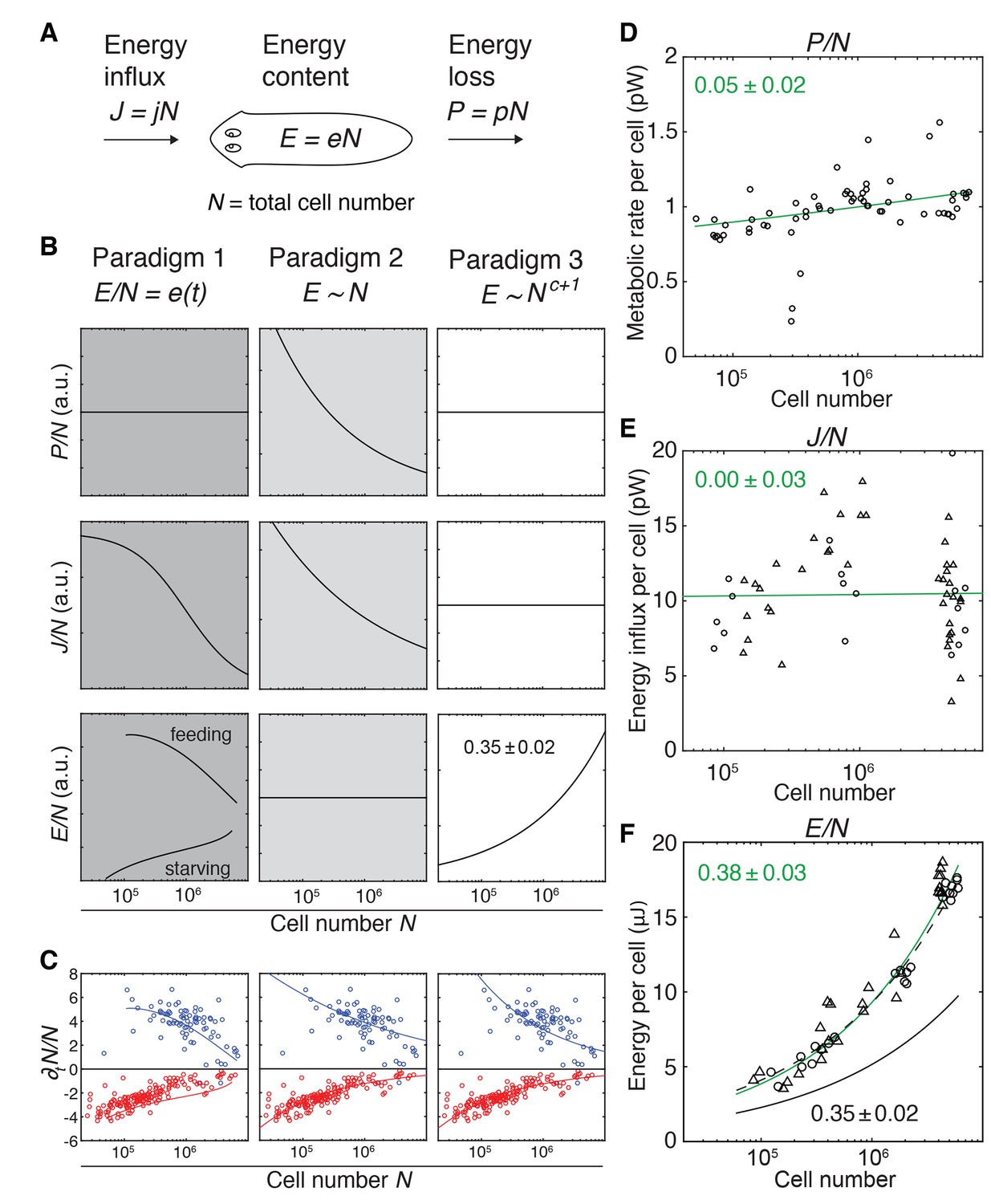
(A) Planarian energy balance model. At the organismal level, changes in the physiological energy content E result from a change in the net energy influx J (feeding) and/or heat loss P (metabolic rate). Dividing E, J and P by the total cell number N approximates the energy balance on a per-cell basis. (B) Three hypothetical control paradigms of E during growth and degrowth (columns), which make specific predictions regarding the size-dependence of *J/N*, *E/N* and *P/N* (rows). Prediction traces and scale exponents were generated by modelling the measured growth/degrowth rates (Figure 2E) with the indicated control paradigm assumptions (see also Appendix 1 and Figure 3—figure supplement 1). (C) Fit of the three control paradigms to the measured growth/degrowth rates (Figure 2E). (D) Metabolic rate per cell (*P/N*) versus organismal cell number (N). Data points were derived by conversion of the measurements from the metabolic rate/dry mass scaling law (Figure 1—figure supplement 1B) via the measured cell number/plan area (Figure 2B) and plan area/dry mass conversion laws (Figure 3—figure supplement 2A). The scaling exponent ± standard error was derived from the respective linear fit (green line) and represents the exponent b of the power law *y = ax^b*. (E) Energy influx per cell versus organismal cell number (N). Data points reflect single-animal quantifications of ingested liver volume per plan area as shown in Figure 3—figure supplement 2B–D, converted into energy influx/cell using the plan area/cell number scaling law (Figure 2B) and the assumption that 1 µl of liver paste corresponds to 6.15 J (USDA Agricultural Research Service, 2016; Overmoyer et al., 1987). Circles, 2 weeks starved and triangles, 3 weeks starved animals. The scaling exponent ± standard error was derived from linear fits (green line) and represents the exponent b of the power law *y = ax^b*. (F) Energy content per cell (*E/N*) versus organismal cell number (N). Data points reflect bomb calorimetry quantifications of heat release upon complete combustion of size matched cohorts of known dry mass as shown in Figure 3—figure supplement 2E, converted via the measured cell number/plan area (Figure 2B) and plan area/dry mass conversion laws (Figure 3—figure supplement 2A). Circles, 1 week starved and triangles, 3 weeks starved animals. The scaling exponent ± standard error was derived from a linear fit (green line) to the data and represents the exponent b of the power law *y = ax^b*. Solid black line, prediction from model three for the physiological energy content per cell assuming a constant metabolic rate *P/N* = 1 pW. Dashed line corresponds to respective prediction under the assumption that the physiological energy (solid black line) amounts to 50% of combustible gross energy in the animal. See Figure 3—source data 1 for numerical data of (C)-(F).

https://doi.org/10.7554/eLife.38187.017

Figure 3—source data 1 Numerical data for Figure 3.: https://doi.org/10.7554/eLife.38187.021
Download elife-38187-fig3-data1-v1.xlsx

Figure 3—figure supplement 1

Download asset Open asset

Further explanation of model paradigm 1.

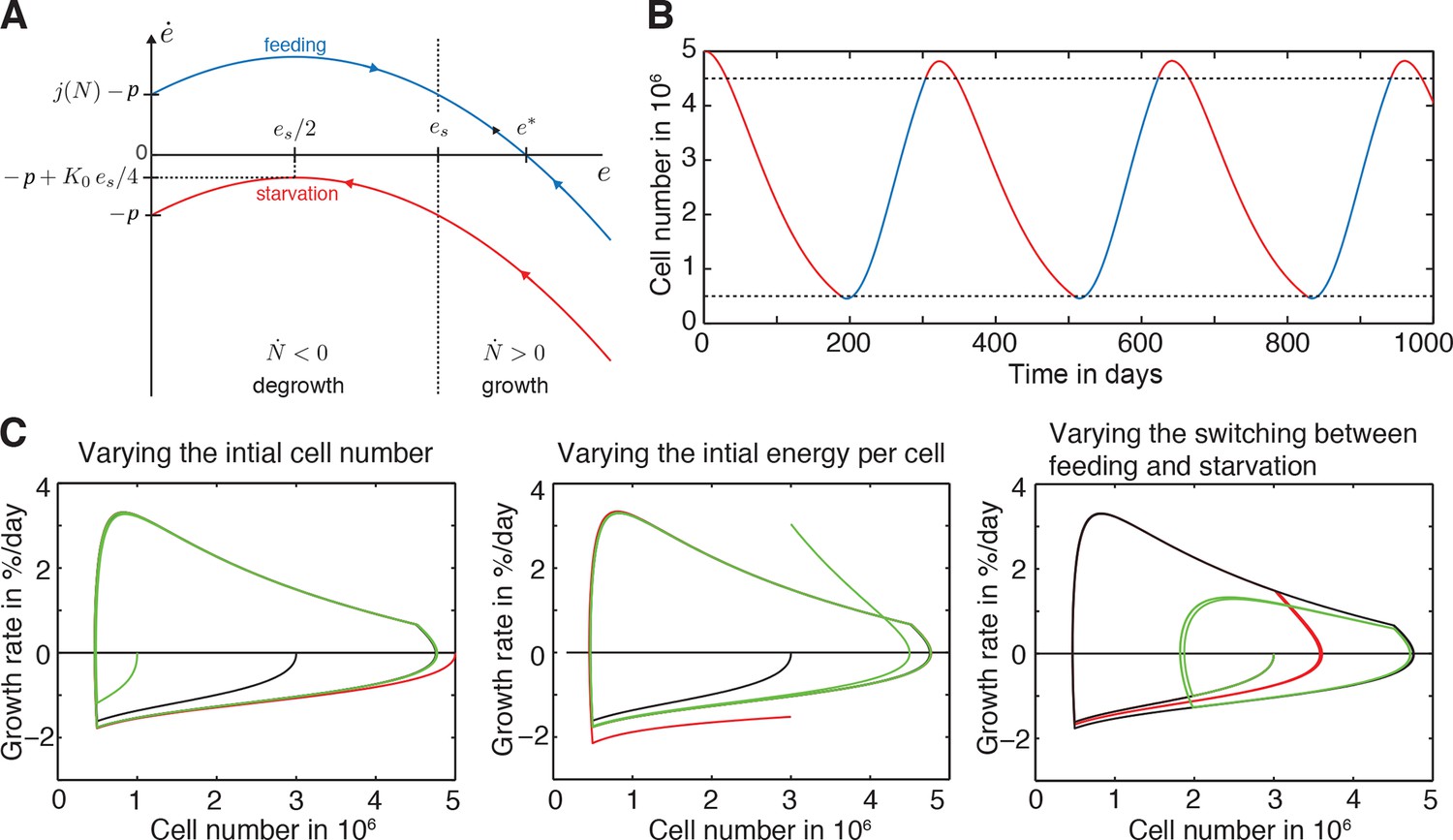
(A) Dynamic behaviour of the energy content per cell during feeding and starvation in paradigm 1. Graph shows the change of the energy content per cell ė as a function of the energy content per cell e during starvation and feeding. See *Appendix 1* for a detailed description of paradigm 1. (B) Time course of the organismal cell number N when going through several rounds of feeding (blue) and starvation (red), always switching at a certain size, specifically at N = 0.5 ∙ 10⁶ cells and N = 4.5 ∙ 10⁶ cells (lower and upper dashed lines, respectively). In the beginning of the starvation interval, we see an overshoot where the animal still grows although feeding has stopped. (C) A generic growth/degrowth dynamic is observed irrespective of the initial cell number, initial energy content or the feeding scheme. Any perturbation decays quickly and there is no strong dependence on feeding history. See Appendix 1 for details.

https://doi.org/10.7554/eLife.38187.018

Figure 3—figure supplement 2

Download asset Open asset

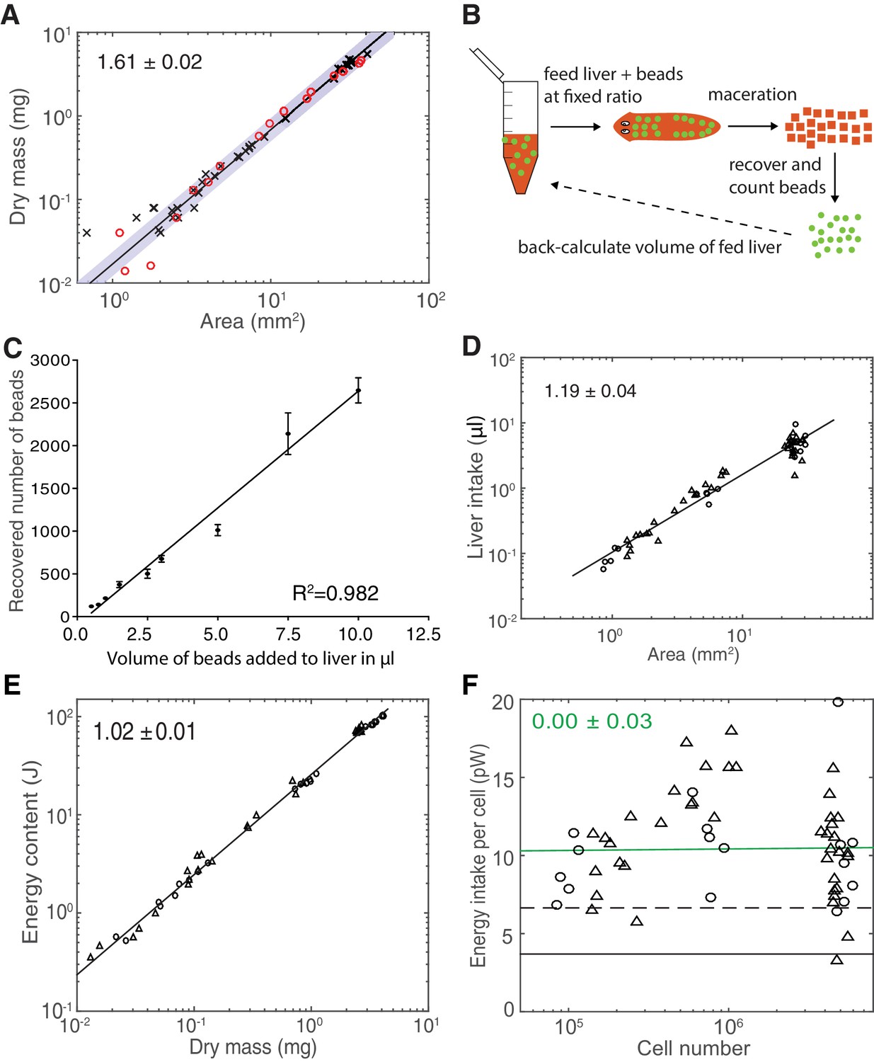
Validation of model paradigms.

(A) Determination of dry mass versus plan area scaling. Each data point represents a single animal measurement, either starved for 1–2 weeks (black crosses) or for 3 weeks (red circles). The fact that both data sets follow the same scaling law indicates no long-term effect of feeding history on the dry mass versus area scaling relationship. The scaling exponent ± standard error was derived from a linear fit (green line, data plotted on logarithmic axes) to the 1–2 weeks starved data and represents the exponent b of the power law *y = ax^b*. These data were further used for the conversion of dry mass into cell numbers via the cell number/area scaling law in Figure 2B and for the extrapolation of the dry mass of an animal of maximal size as in Figure 2—figure supplement 1E, which motivated the up to 9000-fold range in dry mass stated in the discussion. (B) Cartoon illustration of the food intake assay. A mixture of liver (red) with a known concentration of spiked-in fluorescent volume tracer beads (green) was fed to test subjects under *ad libitum* feeding conditions. The subsequent maceration of individual animals immediately after cessation of feeding and bead counting by automated image analysis in a known volume fraction of the macerate allowed extrapolation of the total number of ingested beads and, based on the known bead concentration, the total volume of ingested liver. (C) Titration experiment with different bead concentrations in the food paste. The close match between recovered bead counts and the employed linear dilution scheme (R² = 0.982) demonstrates the quantitative detection of the volume tracer beads in the macerates and thus the validity of the assay. The line represents a fitted linear regression to data from one experiment; error bars represent the standard deviation. Size-matched animals were used as test subjects. (D) Volume of liver ingestion under *ad libitum* feeding conditions as a function of plan area. Data points represent measurements on individual animals, starved for 2 weeks (circles) or 3 weeks (triangles) prior to the experimental feeding. The scaling exponent ± standard error was derived from a linear fit (black line, data plotted on logarithmic axes) and represents the exponent b of the power law *y = ax^b*. The close fit independent of starvation duration demonstrates the history independence of the food intake. The food intake volume and plan are measurements of this experiment were further used to calculate the energy influx per cell, relying on a reported nutritional value of calf liver (USDA Agricultural Research Service, 2016) the density of human adult liver (Overmoyer et al., 1987) and the cell number/area scaling law in Figure 2B. (E) Energy content (gross calorific value) as measured by bomb calorimetry as a function of dry mass. Individual data points represent average energy content and dry mass as obtained by dividing the measured total energy content and dry mass of size-matched cohorts by the number of animals within the cohort. Circles represent 1 week and triangles 3 weeks starved animals and the lack of a difference between the conditions illustrates a lack of feeding history dependence. The scaling exponent ± standard error was derived from a linear fit (black line, data plotted on logarithmic axes) and represents the exponent b of the power law *y = ax^b*. See Figure 3—figure supplement 2—source data 1for data of (A), (D) and (E). These data were further used to determine the energy content per cell via the dry mass/area (A) and cell number/area (Figure 2B) scaling laws. (F) Energy influx per cell versus organismal cell number (N) (same data as shown in in Figure 3E). Data points reflect single-animal quantifications of ingested liver volume per plan area as shown above in Figure 3—figure supplement 2D, converted into energy influx/cell using the plan area/cell number scaling law (Figure 2B) and the assumption that 1 µl of liver paste corresponds to 6.15 J (USDA Agricultural Research Service, 2016; Overmoyer et al., 1987). Green line, fit to the data and representing the gross energy influx/cell based on the total amount of energy contained in the ingested liver volume divided by the organismal cell number. The scaling exponent ± standard error was derived from a linear fit and represents the exponent b of the power law *y = ax^b*. The black dashed line represents the net influx of energy which is assimilated by the animal body per unit cell (~50% of the gross energy influx/cell) following digestion in the intestine and taking into account the use of energy for digestion itself. It is predicted from the conversion between gross and physiological energy (factor of 1.8, see Figure 3F) and corresponds to a feed conversion ratio (ratio between feed mass and resulting gain in body mass, a measure for how efficient an organism converts feed into body mass) of ~2.1, similar to other aquatic animals (Tacon and Metian, 2008), see also discussion. The black solid line represents the physiological net energy influx as predicted from Figure 3D, assuming a constant metabolic rate per cell of 1 pW (~30% of the gross energy influx). It represents the net amount of energy assimilated by the animal body which is fully metabolised and thus contributing to the measured heat production (as given by Figure 3D). Consequently, it constitutes all the energy added during growth which later on can be fully metabolised again (e.g. during starvation). Circles, 2 weeks starved and triangles, 3 weeks starved animals.

https://doi.org/10.7554/eLife.38187.019

Figure 3—figure supplement 2—source data 1 Numerical data for Figure 3—figure supplement 2.: https://doi.org/10.7554/eLife.38187.020
Download elife-38187-fig3-figsupp2-data1-v1.xlsx

Figure 4 with 1 supplement

Download asset Open asset

Size-dependence of lipid and glycogen storage.

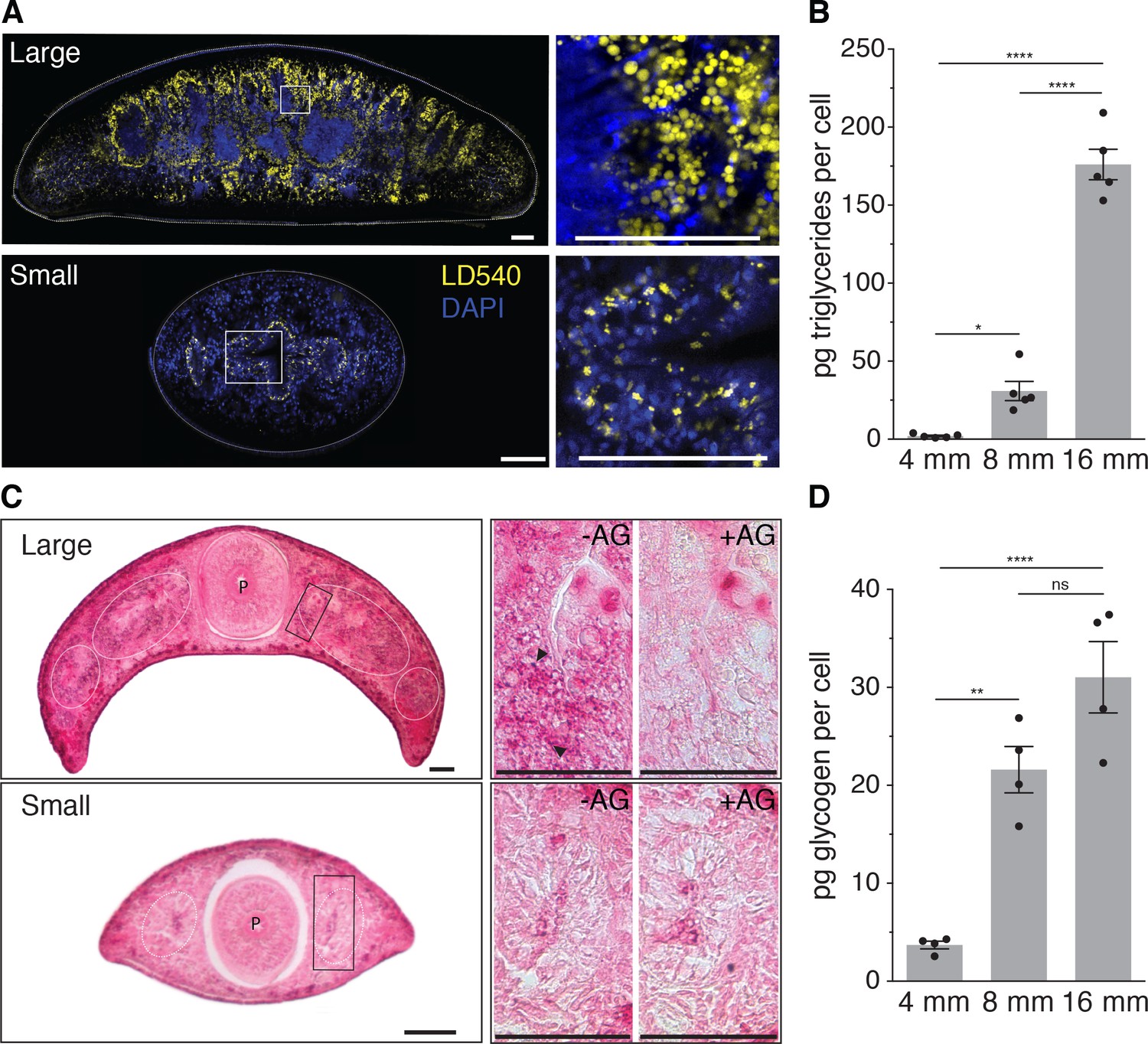
(A) Lipid droplet (LD540, yellow) (Spandl et al., 2009) and nuclei (DAPI, blue) staining of pre-pharyngeal transverse cross sections of a large (16 mm length, top left) and a small (4 mm, bottom left) planarian. Right, magnified view of the boxed areas to the left. Scale bars, 100 µm. See Figure 4—source data 1 for raw images. (B) Mass spectrometry-based quantification of triglycerides in animals of the indicated size (Figure 4—figure supplement 1A–B). All values were normalized to organismal cell numbers using the previously established length versus area (Figure 2—figure supplement 1E) and *N/A* (Figure 2B) scaling laws. Bars mark mean ± SEM. n = 5 biological replicates consisting of 40 pooled 4 mm, 20 8 mm and 6 16 mm long animals analysed in two technical replicates. Significance assessed by one-way ANOVA, followed by Tukey’s post-hoc test (**p_adj* ≤ 0.05, *****p_adj* ≤ 0.0001). See Figure 4—source data 2 for numerical data and statistics. (C) Histological glycogen staining (Best’s Carmine method) of pharyngeal transverse cross sections of a large (16 mm, top left) and a small (4 mm, bottom left) planarian. White circles: outline of intestine branches. P: Pharynx. Right, magnified view of the boxed areas to the left (black rectangles).+AG, pre-treatment with amyloglucosidase, which degrades glycogen; -AG, no pre-treatment of adjacent section. Arrow heads point to small, densely staining glycogen granules. Scale bars, 100 µm. See Figure 4—source data 1 for raw images. (D) Quantification of organismal glycogen content using an enzyme-based colorimetric assay in animals of the indicated length (Figure 4—figure supplement 1D–F). Bars mark mean ± SEM. n = 4 biological replicates (independent experiments), 40 pooled 4 mm, 20 8 mm, 8 16 mm analysed in three technical replicates. Significance assessed by one-way ANOVA, followed by Tukey’s post-hoc test (ns not significant, ***p_adj* ≤ 0.01, *****p_adj* ≤ 0.0001). See Figure 4—source data 2 for numerical data and statistics.

https://doi.org/10.7554/eLife.38187.022

Figure 4—source data 1 Raw images lipid droplet and glycogen.: https://doi.org/10.7554/eLife.38187.024
Download elife-38187-fig4-data1-v1.zip
Figure 4—source data 2 Raw data lipid mass spectrometry, glycogen assay and statistics tables.: https://doi.org/10.7554/eLife.38187.025
Download elife-38187-fig4-data2-v1.xlsx

Figure 4—figure supplement 1

Download asset Open asset

Assays for lipid and glycogen quantification in planarians.

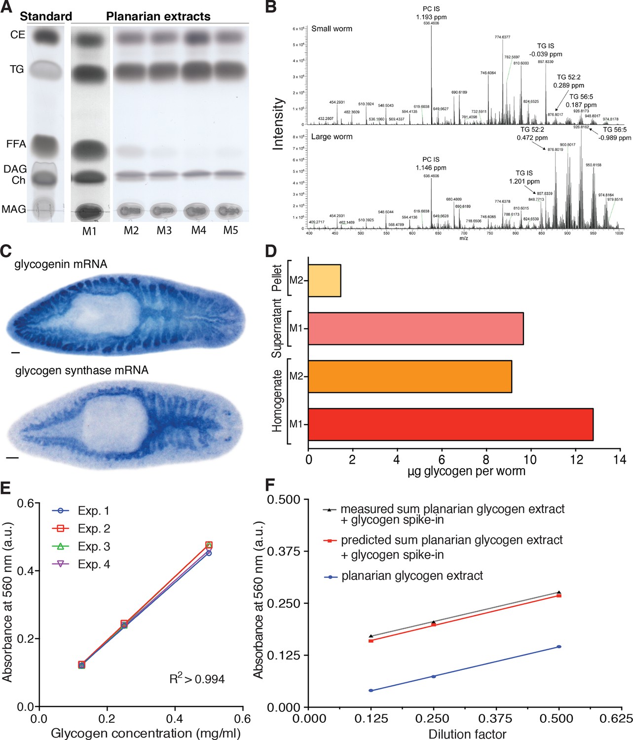
(A) TLC (thin layer chromatography) analysis of planarian lipid extracts under different homogenization conditions to illustrate differences in the level of triglyceride (TG) degradation: M1, Bligh and Dyer method (Bligh and Dyer, 1959); M2, 300 µl isopropanol; M3, 1 ml ice-cold isopropanol; M4, ice-cold isopropanol/acetonitrile (1:1); M5, 1 ml isopropanol with 0.5% glacial acetic acid. Homogenization M4 near-quantitatively prevents TG degradation in the samples, as illustrated by the near complete lack of free fatty acids (FFAs) and the most intense TG band. Therefore, this homogenization procedure was chosen to extract lipids for the mass spectrometry-based quantification of TG. Left, TLC separation of the standards used to identify the lipid species in the planarian samples: CE, Cholesteryl linoleate; TG, Glyceryl trioleate; FFA, Linoleic acid; DAG, Dioleoylglycerol; Ch, Cholesterol; MAG, 1-Oleoyl-rac-glycerol. (B) Representative example of a mass spectrum of small (top) and large animals (bottom) obtained via mass spectrometry (positive ionization mode). Highlighted are the internal standards for Phosphatidylcholine (PC IS) and Triglyceride (TG IS) as well as two of the endogenous planarian triglycerides (TG 52:2 and TG 56:5). The peak intensity of TG 52:2 and TG 56:5 is almost 14-fold higher in large worms compared to small worms while the intensity of PC IS and TG IS show only minor differences (~1.3 fold small vs. large). ppm, parts per million mass accuracy. See Figure 4—source data 2 for quantification of relevant lipid classes. (C) Whole mount in situ hybridization to visualize the expression of *Smed-glycogenin* (top) and *Smed-glycogen synthase* (bottom). The prominent intestinal expression of both core components of glycogen synthesis confirms sugar storage in the form of glycogen in the planarian intestine (see also Figure 4C–D). Scale bars: 100 µm. (D) Comparison of glycogen recovery between two commonly used extraction methods (M1: water; and M2: hot alkali) and different preparation stages (initial homogenate and supernatant versus pellet of a subsequent centrifugation step). Glycogen content was assed via enzymatic break down into glucose using amyloglucosidase and subsequent colorimetric detection of glucose by a colorimetric glucose assay kit. The M1/supernatant combination was chosen for all subsequent experiments, because water extractions consistently yielded high glycogen measurements and the use of the supernatant rather than initial homogenate proved more consistent (not shown). The shown data are from one representative experiment and represent the mean of 3 technical replicates. (E) Standard curves used for the colorimetric glycogen quantification shown in Figure 4D established by the measurement of a linear dilution series of a glycogen standard. The lines represent linear regressions fitted to the data of each experiment (n = 4 independent experiments, three technical replicates each) and the close correspondence between the experiments demonstrates the reproducibility of the assay. (F) Measured glycogen content in a linear dilution series of a glycogen-containing planarian extract (blue line), measured glycogen content in the same extract supplemented with exogenous glycogen (0.16 µg/ul) (dotted grey line) and predicted glycogen content of the supplemented series (red line). The parallel slopes of all three lines demonstrate the linearity of the assay across the entire concentration range and the close correspondence between measured and predicted values demonstrates the absence of interfering substances in the extracts. The lines represent fitted linear regressions (n = 1 experiment, three technical replicates).

https://doi.org/10.7554/eLife.38187.023

Figure 5 with 1 supplement

Download asset Open asset

Size-dependent energy storage explains Kleiber’s law scaling.

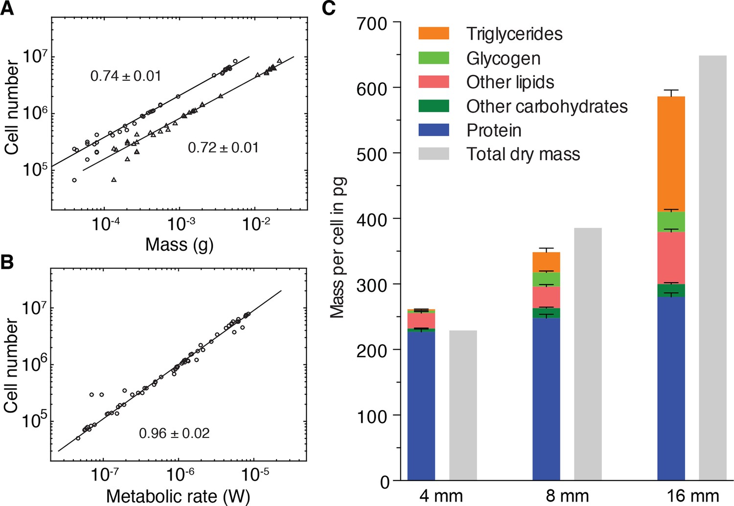
(A) Cell number versus dry mass (circles) or wet mass (triangles) based on the data from Figure 3—figure supplement 2A. Cell numbers were converted from area using the *N/A* scaling law (Figure 2B). Dry and wet mass conversion is given by Figure 1B. Scaling exponents ± standard errors were derived from respective linear fits and represent the exponent b of the power law *y = ax^b* (B) Cell number versus metabolic rate, derived from Figure 1C with scaling laws of Figure 2B and Figure 3—figure supplement 2A. The scaling exponent ± standard error was derived from respective linear fits and represents the exponent b of the power law *y = ax^b*. (C) Mass composition (coloured) and total dry mass (grey) per cell in animals of the indicated body length. Triglyceride and glycogen measurements are taken from Figure 4B and D, respectively. Quantification of other (polar and non-polar) lipids is based on the mass-spectrometry data from Figure 4B (see also Figure 4—figure supplement 1B) (n = 5 biological replicates; p_adj = 0.1720 (no significance) 8 vs. 4 mm, p_adj < 0.0001 16 vs. 4 mm, p_adj < 0.0001 16 vs. 8 mm; two technical replicates). Other carbohydrates represent total carbohydrate minus glycogen. n = 4 biological replicates (independent experiments), 40 pooled 4 mm, 20 8 mm, 8 16 mm long animals; p_adj = 0.0047 8 vs. 4 mm, p_adj = 0.0005 16 vs. 4 mm, p_adj = 0.2790 16 vs. 8 mm; three technical replicates. Protein content was measured colorimetrically. n = 4 biological replicates (independent experiments), 44 pooled 4 mm, 10 8 mm, 10 16 mm long animals; p_adj = 0.0020 8 vs. 4 mm, p_adj < 0.0001 16 vs. 4 mm, p_adj = 0.0007 16 vs. 8 mm) (see also Figure 5—figure supplement 1). Significance was assessed by one-way ANOVA followed by Tukey’s post-hoc test. All values were normalised to the total cell number using the previously established length-area (Figure 2—figure supplement 1E) and N/A (Figure 2B) scaling laws. Total dry mass was independently measured (Figure 3—figure supplement 2A) and correlated with length using the length-area relationship (Figure 2—figure supplement 1E). All values are shown as mean ± SEM. See Figure 5—source data 1 for numerical data and statistics.

https://doi.org/10.7554/eLife.38187.026

Figure 5—source data 1 Raw data and statistics tables for measurement of other lipids, carbohydrates and protein.: https://doi.org/10.7554/eLife.38187.028
Download elife-38187-fig5-data1-v1.xlsx

Figure 5—figure supplement 1

Download asset Open asset

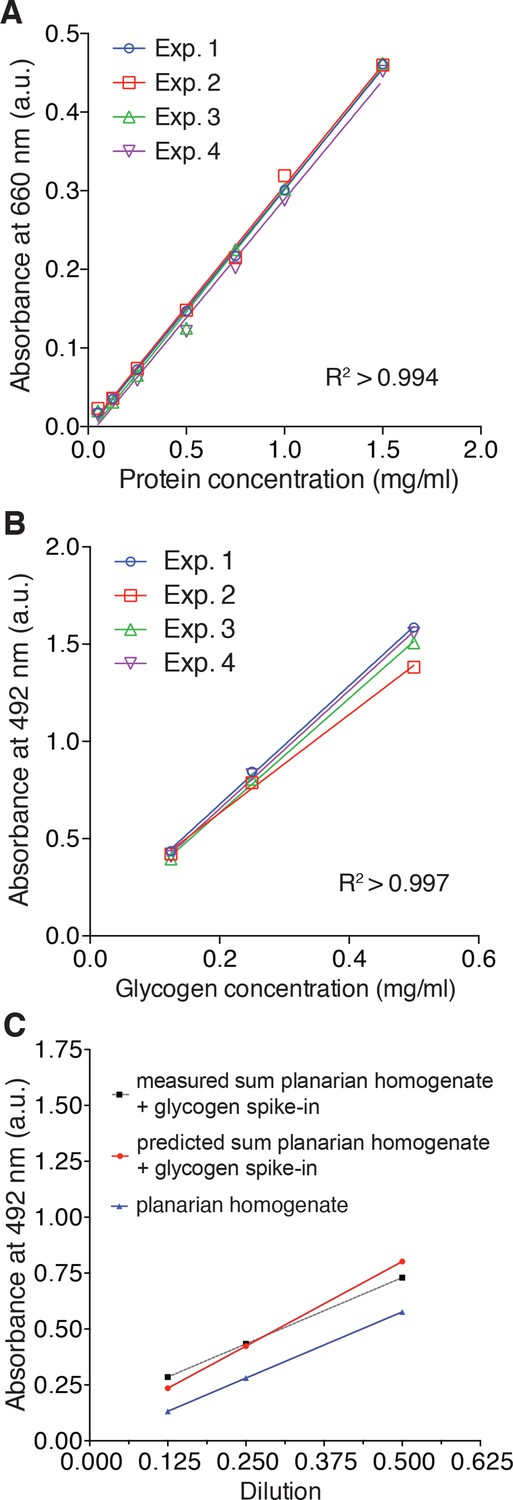
Validation of protein and total carbohydrate quantifications.

(A) Standard curves used for the colorimetric protein quantification by the Pierce 660 nm Protein Assay shown in Figure 5C. The lines represent linear regressions fitted to a series of standard dilutions of a test protein (bovine serum albumin) prepared de novo for each experiment (n = 4 independent experiments, three technical replicates). (B) Standard curves for the total carbohydrate content quantification in Figure 5C by the colorimetric phenol-sulfuric acid method. The lines represent linear regressions fitted to a series of standard dilutions of a glycogen standard prepared de novo for each experiment (n = 4 independent experiments, three technical replicates). (C) Measured total carbohydrate content of a linear dilution series of a carbohydrate containing planarian extract (blue line), measured total carbohydrate content of the same extract supplemented with exogenous glycogen (conc. = 0.25 µg/µl) (dotted grey line) and predicted total carbohydrate content of the supplemented series (red line). The largely parallel slopes of all three lines demonstrate the linearity of the assay across the entire concentration range and the close correspondence between measured and predicted values demonstrates a lack of interfering substances in the extracts. The lines represent fitted linear regressions (n = 1 experiment, three technical replicates).

https://doi.org/10.7554/eLife.38187.027

Tables

Key resources table

Reagent type (species) or resource	Designation	Source or reference	Identifiers	Additional information
Strain (Schmidtea mediterranea)	asexual CIW4 strain of Schmidtea mediterranea	other	NA	obtained from Dr. Alejandro Sánchez Alvarado (Stowers Institute, Kansas City, USA)
Chemical compound, drug	FluoSpheres Sulfate Microspheres 4 µm, red fluorescent 580/605 nm	ThermoFisher Scientific	ThermoFisher Scientific: F8858	See materials and methods
Chemical compound, drug	FluoSpheres Sulfate Microspheres 4 µm, yellow-green fluorescent 505/515 nm	ThermoFisher Scientific	ThermoFisher Scientific: F8859	See materials and methods
Chemical compound, drug	LD540 lipid droplet stain	Spandl et al., 2009	NA	obtained from Dr. Christoph Thiele (LiMES, Universität Bonn, Germany)
Chemical compound, drug	Bouins fixative	TCS Biosciences	TCS Biosciences: A1602	See materials and methods
Chemical compound, drug	Amyloglucosidase; AG	Sigma-Aldrich	Sigma-Aldrich: A1602	See materials and methods
Chemical compound, drug	Carmine (C.I. 75470)	Carl Roth	Carl Roth: 6859.1	See materials and methods
Chemical compound, drug	Richard-Allan Scientific Cytoseal XYL	ThermoFischer Scientific	ThermoFischer Scientific: 8312–4	See materials and methods
Chemical compound, drug	Benzoic acid pellets; IKA C723	IKA	IKA: 0003243000	See materials and methods
Chemical compound, drug	Lipid standard: CE 16:0 D7	Avanti Polar Lipids	Avanti Polar Lipids: 700149	See materials and methods
Chemical compound, drug	Lipid standard: CholD7	Avanti Polar Lipids	Avanti Polar Lipids: 700041	See materials and methods
Chemical compound, drug	Lipid standard: TAG 50:0 D5	Avanti Polar Lipids	Avanti Polar Lipids: 110543	See materials and methods
Chemical compound, drug	Lipid standard: DAG 34:0 D5	Avanti Polar Lipids	Avanti Polar Lipids: 110538	See materials and methods
Chemical compound, drug	Lipid standard: Cer 30:1	Avanti Polar Lipids	Avanti Polar Lipids: 860512	See materials and methods
Chemical compound, drug	Lipid standard: PC 25:0	Avanti Polar Lipids	Avanti Polar Lipids: LM-1000	See materials and methods
Chemical compound, drug	Lipid standard: PE 25:0	Avanti Polar Lipids	Avanti Polar Lipids: LM-1100	See materials and methods
Chemical compound, drug	Lipid standard: PS 25:0	Avanti Polar Lipids	Avanti Polar Lipids: 111129	See materials and methods
Chemical compound, drug	Lipid standard: PI 25:0	Avanti Polar Lipids	Avanti Polar Lipids: 110955	See materials and methods
Chemical compound, drug	Lipid standard: SM 30:1	Avanti Polar Lipids	Avanti Polar Lipids: 860583	See materials and methods
Chemical compound, drug	Lipid standard: LPC 13:0	Avanti Polar Lipids	Avanti Polar Lipids: 855476P	See materials and methods
Chemical compound, drug	Lipid standard: LPE 13:0	Avanti Polar Lipids	Avanti Polar Lipids: 110696	See materials and methods
Chemical compound, drug	Lipid standard: PG 25:0	Avanti Polar Lipids	Avanti Polar Lipids: 111126	See materials and methods
Chemical compound, drug	Lipid standard: PA 25:0	Avanti Polar Lipids	Avanti Polar Lipids: LM-1400	See materials and methods
Chemical compound, drug	Lipid standard: LPA 13:0	Avanti Polar Lipids	Avanti Polar Lipids: LM-1700	See materials and methods
Chemical compound, drug	Lipid standard: GalCer 30:1	Avanti Polar Lipids	Avanti Polar Lipids: 860544	See materials and methods
Chemical compound, drug	Lipid standard: LacCer 30:1	Avanti Polar Lipids	Avanti Polar Lipids: 860545	See materials and methods
Chemical compound, drug	Lipid standard: LPI 13:0	Avanti Polar Lipids	Avanti Polar Lipids: 110716	See materials and methods
Chemical compound, drug	Cholesteryl linoleate	Sigma-Aldrich	Cat. No.: C0289	See materials and methods
Chemical compound, drug	Glyceryl trioleate	Sigma-Aldrich	Cat. No.: T7140	See materials and methods
Chemical compound, drug	Linoleic acid	Sigma-Aldrich	Cat. No.: L1376	See materials and methods
Chemical compound, drug	Dioleoylglycerol	Sigma-Aldrich	Cat. No.: D8894	See materials and methods
Chemical compound, drug	Cholesterol	Sigma-Aldrich	Cat. No.: C8503	See materials and methods
Chemical compound, drug	1-Oleoyl-rac-glycerol	Sigma-Aldrich	Sigma, Cat. No.: M7765	See materials and methods
Antibody	anti-Histone H3	Abcam	Cat. No.: ab1791	(1:500)
Antibody	anti-rabbit IRDye 680LT	LICOR	Cat. No.: 926–68023	(1:20000)
Commercial assay or kit	Glucose (GO) Assay Kit	Sigma-Aldrich	Cat. No.: GAGO-20	See materials and methods
Commercial assay or kit	Protein Assay Reagent	ThermoFischer Scientific	Cat. No.: 22660	See materials and methods
Commercial assay or kit	Detergent Compatibility Reagent	ThermoFischer Scientific	Cat. No.: 22663	See materials and methods
Other	microcalorimeter TAMIII	TA Instruments	NA	See materials and methods
Other	Bomb calorimeter IKA C 6000 global standards	IKA	NA	See materials and methods
Other	Odyssey SA Li-Cor Infrared Imaging System	LICOR	NA	See materials and methods
Software, algorithm (MATLAB)	MATLAB	MathWorks	NA	Algorithm to measure planarian body size available as a source file.
Software, algorithm	Fiji distribution of ImageJ	Schindelin et al. (2012)	NA	See materials and methods
Software, algorithm CellProfiler	CellProfiler (version 2.2.0 and older)	Carpenter et al., 2006	NA	Pipeline used for cell counting available as a source file.