'Artiphysiology' reveals V4-like shape tuning in a deep network trained for image classification
- University of Washington, United States
- University of Washington Institute for Neuroengineering, United States
Figures
Figure 1

The 96 kernels (11 × 11 pixels, by three color channels) of the 1 st layer, Conv1, of the AlexNet model tested here.
Like many V1 receptive fields, many of these kernels are band-limited in spatial frequency and orientation. Each kernel was independently scaled to maximize its RGB dynamic range to highlight spatial structure.
Figure 2
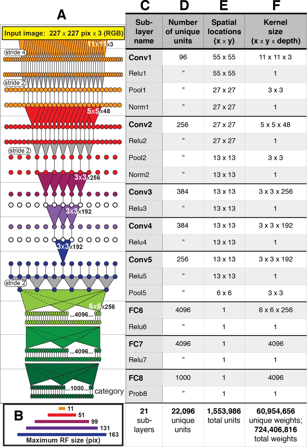
Architecture of the Caffe AlexNet CNN.
(A) A one-dimensional scale view of the fan-in and spatial resolution of units for all 21 sublayers, aligned to their names listed in column (C). The color-filled triangles in convolutional (Conv) layers indicate the fan-in to convolutional units, gray triangles indicate the fan-in to max pooling units, and circles (or ovals) indicate the spatial positions of units along the horizontal dimension. For the Conv layers and their sublayers, each circle in the diagram represents the number of unique units listed in column (D). For example, for each orange circle/oval in the four sublayers associated with Conv1, there are 96 different units in the model (the Conv1 kernels are depicted in Figure 1). The 227 pixel wide input image (top, yellow), is subsampled at the Conv1 sublayer (orange; ‘stride 4’ indicates that units occur only every four pixels) and again at each pooling sublayer (‘stride 2’), until the spatial resolution is reduced to a 6 × 6 grid at the transition from Pool5 to FC6. The pyramid of support converging to the central unit in Conv5 (dark blue triangle) is indicated by triangles and line segments starting from Conv1. Each unit in layers FC6, FC7 and FC8 (shades of green; not all units are shown) receives inputs from all units in the previous layer (there is no spatial dimension in the FC layers, units are depicted in a line only for convenience). Green triangles indicate the full fan-in to three example units in each FC layer. (B) The maximum width (in pixels) of the RFs for units in the five convolutional layers (colors match those in (A)) based on fan-in starting from the input image. For the FC layers, the entire image is available to each unit. (C) Names of the sublayers, aligned to the circuit in (A). Names in bold correspond to the eight major layers, each of which begins with a linear kernel (colorful triangles in (A)). (D) The number of unique units, that is feature dimensions, in each sublayer (double quotes repeat values from previous row). (E) The width and height of the spatial (convolutional) grid at each sublayer, or ‘1’ for the FC layers. The total number of units in each sublayer can be computed by multiplying the number of unique kernels (D) by the number of spatial positions (E). (F) The kernel size corresponds to the number of weights learned for each unique linear kernel. Pooling layers have 3 × 3 spatial kernels but have no weights—the maximum is taken over the raw inputs. The Conv2 kernels are only 48 deep because half of the Conv2 units take inputs from the first 48 feature dimensions in Conv1, whereas the other half take inputs from the last 48 Conv1 features; inputs are similarly grouped in Conv4 and Conv5 (see Krizhevsky et al.'s Figure 2). The bottom row provides totals. In addition to the weights associated with each kernel, there is also one bias value per kernel (not shown), which adds 10,568 free parameters to the 60.9 million unique weights.
Figure 3

The angular position and curvature (APC) model and associated stimuli.
(A) The set of 51 simple closed shapes from Pasupathy and Connor, 2001. Shapes are shown to relative scale. Shape size, given in pixels in the text, refers to the diameter of the big circle (top row, 2nd shape from the left). Each shape was shown at up to eight rotations as dictated by rotational symmetry, e.g., the small and large circles (upper left) were only shown at one rotation. This yielded a set of 362 unique shape stimuli. Stimuli were presented as white-on-black to the network (not as shown here). (B) Example shape with points along the boundary (red circles) indicating where angular position and curvature values were included in the APC model. (C) Points from the example shape in (B) are plotted in the APC plane where x-axis is angular position and y-axis is normalized curvature. Note the red circle furthest to the left at 0° angular position and negative curvature corresponds to the concavity at 0° on the example shape in (B). A schematic APC model is shown (ellipse near center of diagram) that is a product of Gaussians along the two axes. This APC model would describe a neuron with a preference for mild concavities at 135°.
Figure 4 with 1 supplement
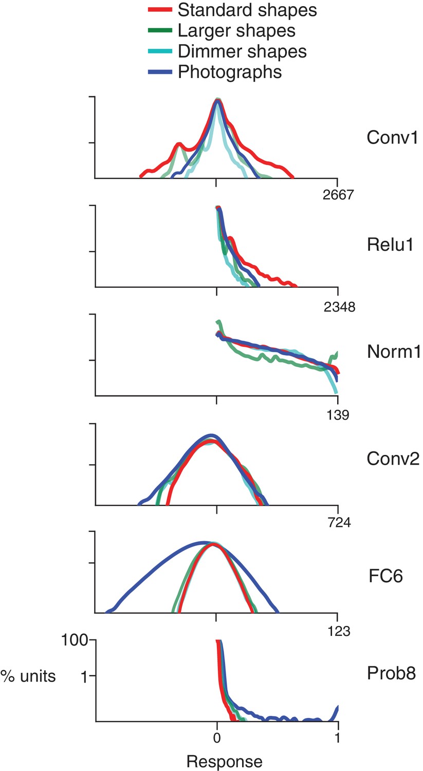
Response distributions for shapes and natural images in representative CNN layers.
In each panel, the frequency distribution of the response values across all unique units in a designated CNN sublayer is plotted for four stimulus sets: our standard shape set (red; size 32 pixels, stimulus intensity 255, see Materials and methods), larger shapes (cyan; size 64 pixels, intensity 255), dimmer shapes (green; intensity 100, size 32 pixels) and natural images (dark blue). Natural images (n = 362, to match the number of shape stimuli) were pulled randomly from the ImageNet 2012 competition validation set. From top to bottom, panels show results for selected sublayers: Conv1, Relu1, Norm1, Conv2, FC6 and Prob8 (Figure 2C lists sublayer names). The number of points in each distribution is given by the number of stimuli (362) times the number of unique units in the layer (Figure 2D). The vertical axis is log scaled as most distributions have a very high peak at 0. For Conv1, standard shapes drove a wider overall dynamic range than did images because of the high intensity edges that aligned with parts of the linear kernels (Figure 1). This was not the case for larger shapes because they often over-filled the small Conv1 kernels. For Relu1, negative responses are removed by rectification after a bias is added. At Conv2, there is little difference between the four stimulus sets on the positive side of the distribution. This changes from FC6 forward, where natural images drive a wider range of responses. For Prob8, natural images (dark blue line) sometimes result in high probabilities among the 1000 categorical units, whereas shapes do not.
Figure 4—figure supplement 1
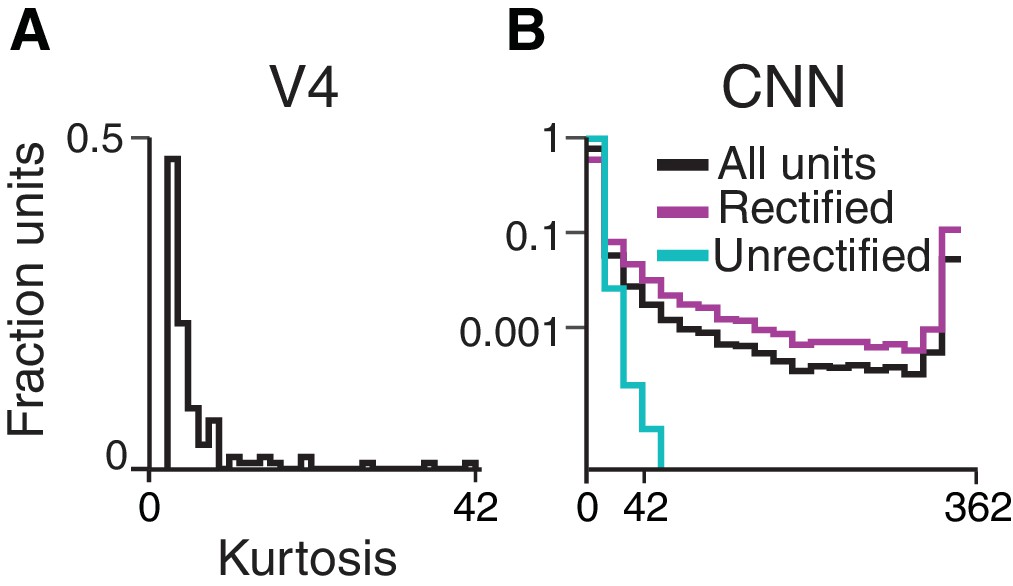
Sparsity of CNN and V4 unit responses to shape stimuli (see end of document).
Figure 5

Boundary curvature selectivity for CNN units compared to V4 neurons.
(A) APC model prediction vs. CNN unit response for an example CNN unit from an early layer (Conv2-113). (B) The top and bottom eight shapes sorted by response amplitude (most preferred shape is at upper left, least at lower right) reveal a preference for convexity to the upper left (such a feature is absent in the non-preferred shapes). This is consistent with the APC fit parameters, , , °, °. (C) Predicted vs. measured responses for another well-fit example CNN unit (FC7-3591) but in a later layer. (D) Top and bottom eight shapes for example unit in (C). The APC model fit was , , °, °. (E) Model prediction vs. neuronal mean firing rate (normalized) for the V4 neuron (a1301) that had the highest APC fit r-value. (F) The top eight shapes (purple) all have a strong convexity to the left, whereas the bottom eight (cyan) do not. The APC model fit was , , °, °. (G) The cumulative distributions (across units) of APC r-values are plotted for the first sublayer of each major CNN layer (boldface names in Figure 2C) from Conv1 (black) to FC8 (lightest orange). The other sublayers (distributions not shown for clarity) tended to have lower APC r-values but the trend for increasing APC r-value with layer was similar. For comparison, red line shows cumulative distribution for 109 V4 neurons (Pasupathy and Connor, 2001), and pink line shows V4 distribution corrected for noise (see Materials and methods). (H) The cumulative distribution of r-values for the APC fits for all CNN units (black), CNN units with shuffled responses (green), units in an untrained CNN (blue) and V4 (red and pink). The far leftward shift of the green line shows that fit quality deteriorates substantially when the responses are shuffled across the 362 stimuli within each unit.
Figure 6
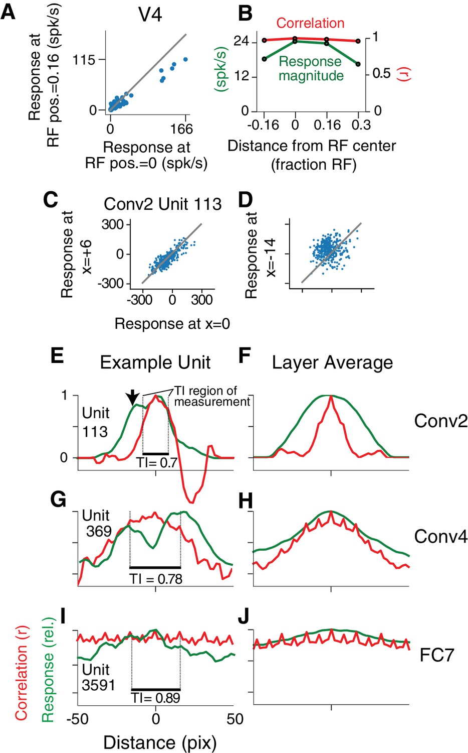
Translation invariance as a function of position across the RF.
(A) For an example neuron from the V4 study of El-Shamayleh and Pasupathy (2016), the responses to stimuli shifted away from the RF center by 1/6 of the estimated RF size are plotted against those placed in the RF center. The overall response magnitude decreases with shift, but a strong linear relationship is maintained between responses at the two positions. (B) In green, the RF profile of the same neuron from (A) is plotted (average response at each position). In red, the correlation of the responses at each position with the responses at RF center. (C) For unit Conv2-113, responses to stimuli shifted six pixels to the right are plotted against responses for centered stimuli. (D) For the same unit in (C), responses for stimuli shifted 14 pixels to the left vs. responses for centered stimuli. (E) For unit Conv2-113, the position-correlation function is plotted in red. The RF profile, that is the normalized response magnitude (square root of sum of squared responses) across all shapes is plotted in green. The region over which TI is measured, where all stimuli are wholly within the CRF (see Materials and methods), is within dotted lines bookending horizontal black bar. The unit is less translation invariant because it continues to have a large response even when correlation drops quickly from center. This is reflected in the lower TI score of 0.7. (F) The averages of the correlation and RF profiles across all units in the Conv2 layer show that correlation drops off much more rapidly than the RF profile. (G) Same as in (E) but for a unit in the 4th convolutional layer (Conv4-369). There is a broadened correlation profile compared to the Conv2 unit. (H) For Conv4, the average position-correlation function (red) has a wider peak than that for Conv2, more closely matching the shape of the average RF profile (green). It also has serrations that occur eight pixels apart, which corresponds to the pixel stride (discretization) of Conv2 (Figure 2A; see Materials and methods). (I) The shape-tuned example unit FC7 3591 (Figure 5C) in the final layer is highly translation invariant (TI = 0.89). (J) The response profile and correlation stay high across the center of the input field on average across units in FC7.
Figure 7 with 1 supplement
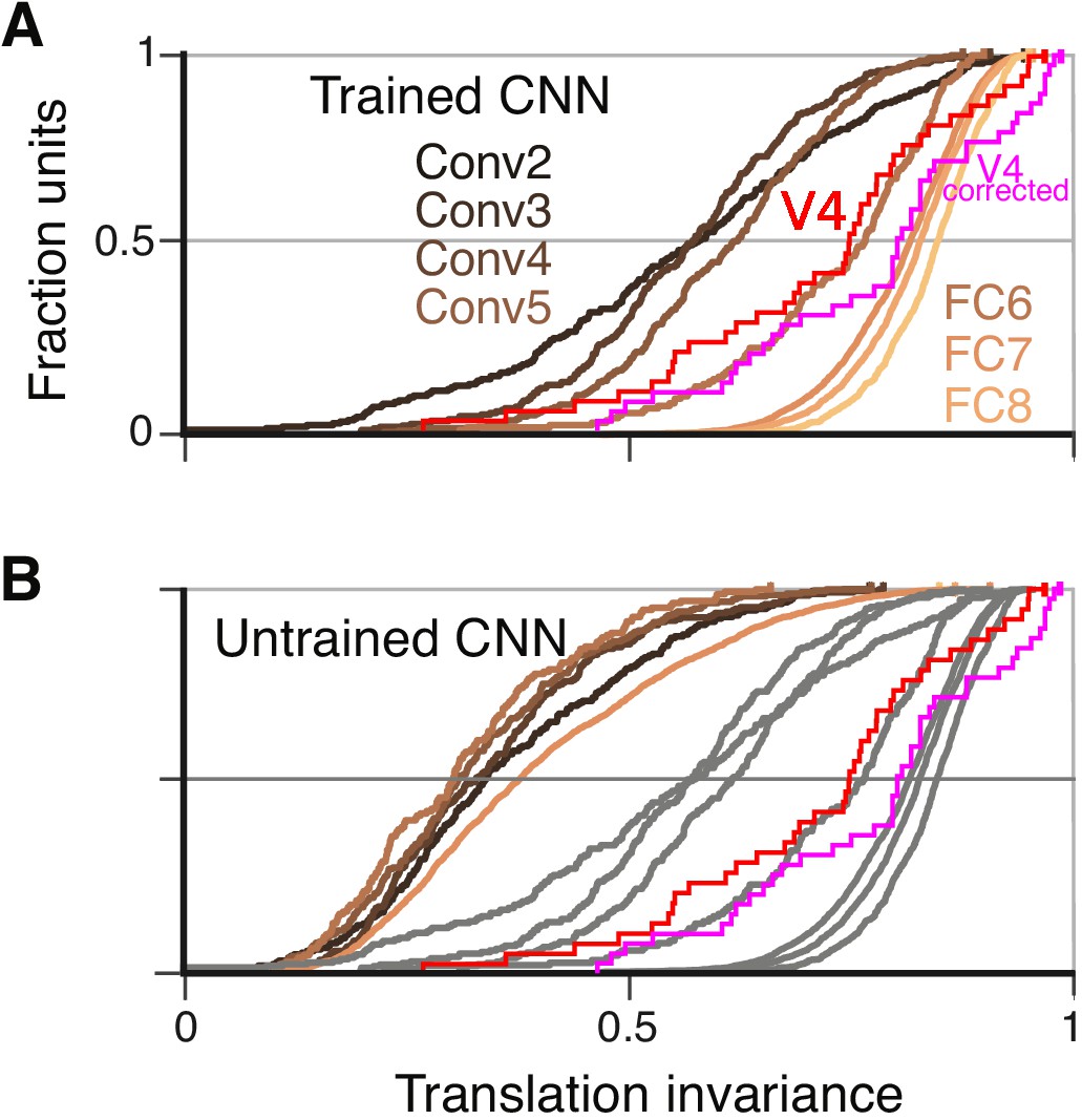
Cumulative distributions of the TI metric for the CNN and V4.
(A) The cumulative distributions (across units) of TI are plotted for the first sublayer of each major CNN layer (boldface names in Figure 2C) from Conv2 (black) to FC8 (lightest orange). There is a clear increase in TI moving up the hierarchy. The TI distribution for V4 is plotted in red, and an upper bound for noise correction is plotted in pink (see Materials and methods). The other sublayers (distributions not shown for clarity) tended to have lower TI values but the trend for increasing TI with layer was similar. (B) The cumulative distribution of TI across layers in the untrained CNN. There is a large shift toward lower TI values in comparison to the trained CNN (faint grey and red and pink lines reproduce traces from panel A).
Figure 7—figure supplement 1
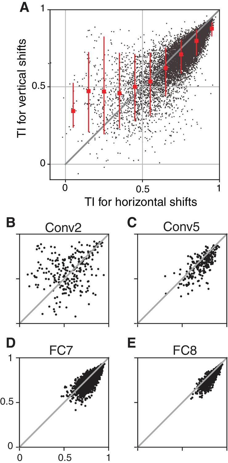
The consistency of translation invariance across sampling directions.
Our tests of translation invariance are based on the TI metric measured for horizontal shifts of the stimuli. High values of the TI metric are meant to indicate which units are generally translation invariant, thus we examined whether a high score for shifts along one direction were associated with a similar score along the orthogonal direction. (A) TI measured for vertical shifts is plotted against TI for horizontal shifts for all CNN units. Points with high TI values are more tightly clustered near the line of equality than are points with lower TI values, indicating that a high TI value measured for horizontal shifts tends to imply a high value for vertical shifts (). We examined this relationship separately for each layer and found that early layers, for example Conv2 (B) contribute most of the highly scattered, low-TI points. As TI improves with deeper layers, the points tend to cluster more tightly on the line of equality and move toward the upper right, as shown for layers Conv5 (C), FC7 (D) and FC8 (E). Interestingly, high TI values in earlier layers are less consistent across axes of translation than in later layers. Such inconsistency is an indication that, in early layers, the selectivity can vary along one axis much more than it does along the other (e.g., a simple cell tuned for horizontal orientation has luminance selectivity that varies more strongly in the vertical dimension than in the horizontal dimension). The consistency of TI values across axes in later layers suggests that their selectivity is spatially more homogeneous. Overall, the high correlation between TI along the x and y axes for units in all but the earliest layers suggests that measuring TI in the x-direction can often be a useful shortcut for approximating the degree of translation invariance without adding a second dimension to the stimulus set. Overall, we found that our conclusions did not vary whether we measure TI in x, in y, or in both dimensions: units in the early CNN layers had TI values lower on average than those found in V4, whereas units in the deeper layers had TI values larger on average than those in V4.
Figure 8
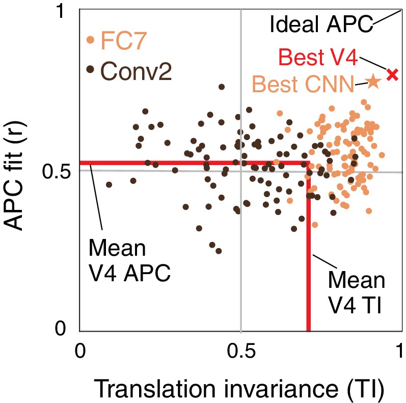
Summary of the similarity of CNN units to V4 neurons in terms of translation invariance (TI) and fit to the APC model.
For 100 randomly selected CNN units from Conv2 (brown) and FC7 (orange), APC r-value is plotted against TI. The hypothetical highest scoring V4 unit (red ×) is the combination of the highest TI score and the highest APC fit from separate V4 data sets (0.97, 0.80). The highest scoring unit in the CNN (FC7-3591, from Figure 5C, Figure 6I and Figure 12C) is indicated by the orange star (0.91, 0.77) and is close to the hypothetical best V4 unit. The red lines indicate the mean V4 values along each axis, not including any correction for noise (see Figures 5 and 7 for estimated noise correction, pink lines).
Figure 9
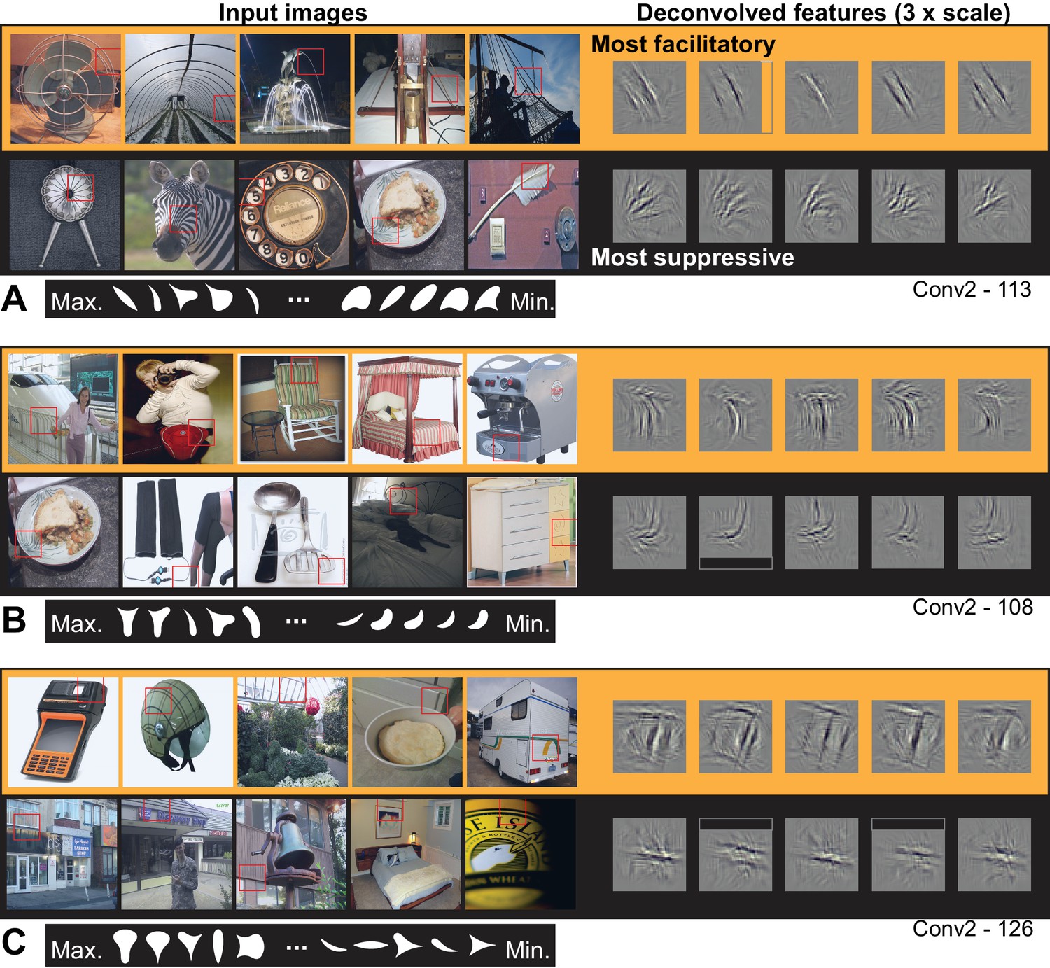
Visualization of APC-like units in layer Conv2.
(A) For unit Conv2-113, the five most excitatory image patches are indicated by red squares superimposed in the raw images (top row, left side, from left to right). The size of the red square corresponds to the maximal extent of the image available to Conv2 units (see Figure 2B). In corresponding order, the five deconvolved features are shown at the upper right, with a 3x scale increase for clarity. The blank rectangular region at the right side of the second feature indicates that this part of the unit RF extended beyond the input image (such regions are padded with zero during response computation). For the same unit, the lower row shows the five most suppressive image patches and their corresponding deconvolved features. We examined the top 10 most excitatory and suppressive images, and for all examples in this and subsequent figures, they were consistent with the top 5. Below the natural images are the top 5 and bottom five shapes (white on black background) in order of response from highest (at left) to lowest (at right). Shapes are shown at 2x scale relative to images, for visibility. (B) Same format as (A), but for unit Conv2-108. (C) Same format as (A), but for unit Conv2-126. In all examples, the most suppressive features (bottom row in each panel) tend to run orthogonal to, and at the same RF position, as the preferred features (top row in each panel) For APC fit parameters, see Table 1 in Results text. Thumbnails featuring people were redacted for display in the published article, in line with journal policy. Input image thumbnails were accessed via the ImageNet database and the original image URLs can be found through this site: http://image-net.org/about-overview.
© 2018, Various. Image thumbnails were taken from http://image-net.org and may be subject to copyright. They are not available under CC-BY and are exempt from the CC-BY 4.0 license.
Figure 10
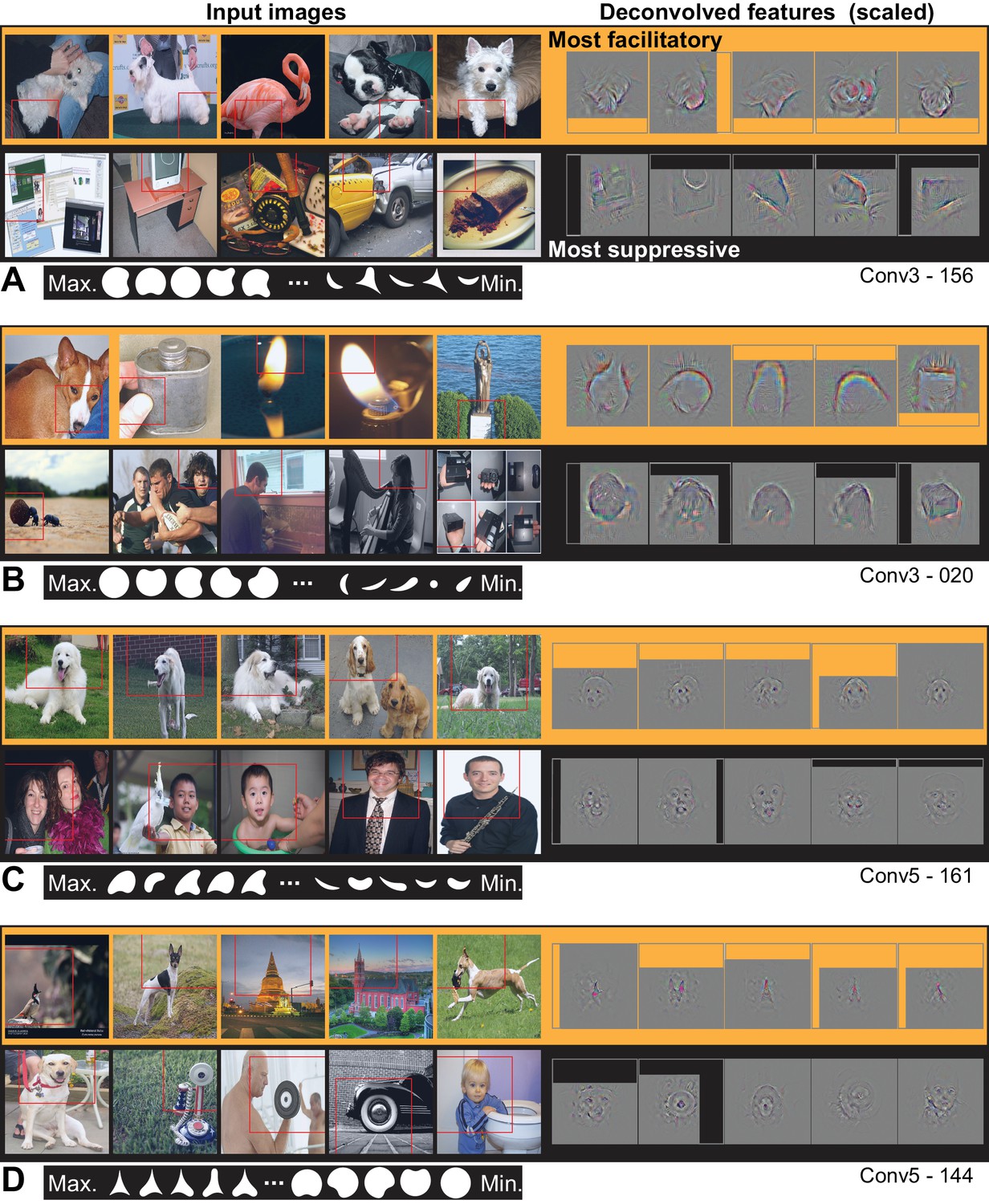
Visualization of APC-like units in layers Conv3 to Conv5.
(A) Visualization for unit Conv3-156, using the same format as Figure 9. Deconvolved features are scaled by 1.8 for visibility. (B) Same as (A), for unit Conv3-020. (C) Same for unit Conv5-161, but deconvolved features are scaled by 1.15. (D) Same as (C), but for unit Conv5-144. For APC fit parameters, see Table 1 in main text. Thumbnails featuring people were redacted for display in the published article, in line with journal policy. Input images were accessed via the ImageNet database and the original image URLs can be found through this site: http://image-net.org/about-overview.
© 2018, Various. Image thumbnails were taken from http://image-net.org and may be subject to copyright. They are not available under CC-BY and are exempt from the CC-BY 4.0 license.
Figure 11
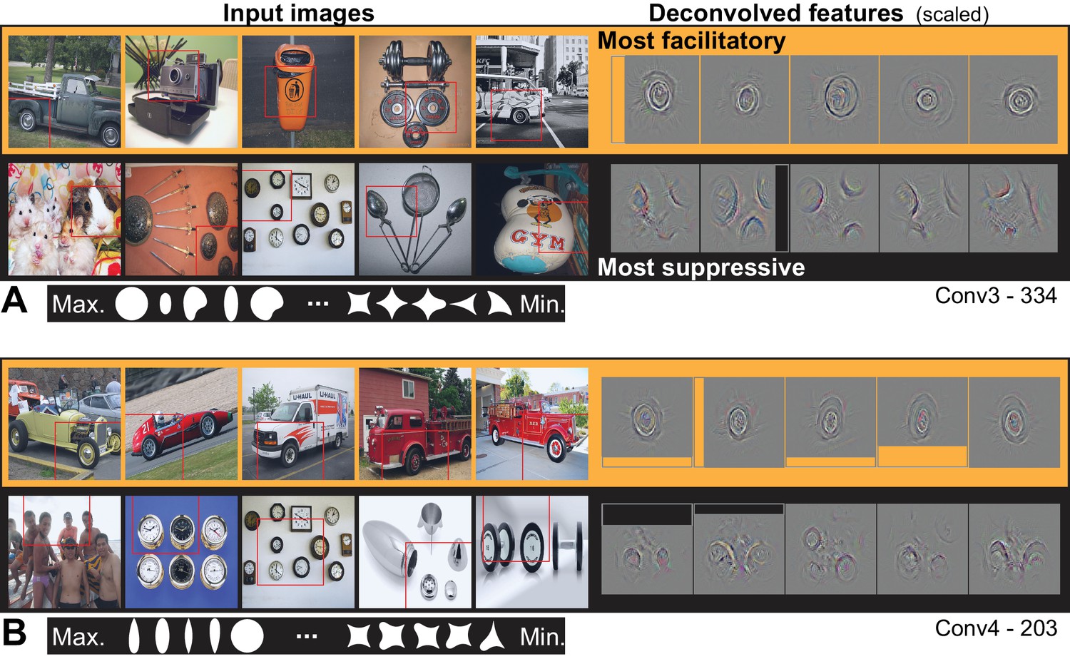
Visualization of APC-like units: circle detectors.
These examples are representative of many units that were selective for circular forms. (A) Unit Conv3-334 was selective for a wide variety of circular objects near its RF center and was suppressed by circular boundaries entering its RF from the surround. Deconvolved feature patches are scaled up by 1.8 relative to raw images. (B) Unit Conv4-203 was also selective for circular shapes near the RF center, but showed category specificity for vehicle wheels. Suppression was not category specific but was, like that in (A), related to circular forms offset from the RF center. The higher degree of specificity in (B) is consistent with this unit being deeper than the example in (A). Deconvolved features are scaled by 1.4 relative to raw images. APC fit parameters are given in Table 1. Thumbnails featuring people were redacted for display in the published article, in line with journal policy. Input images were accessed via the ImageNet database and the original image URLs can be found through this site: http://image-net.org/about-overview.
© 2018, Various. Image thumbnails were taken from http://image-net.org and may be subject to copyright. They are not available under CC-BY and are exempt from the CC-BY 4.0 license.
Figure 12
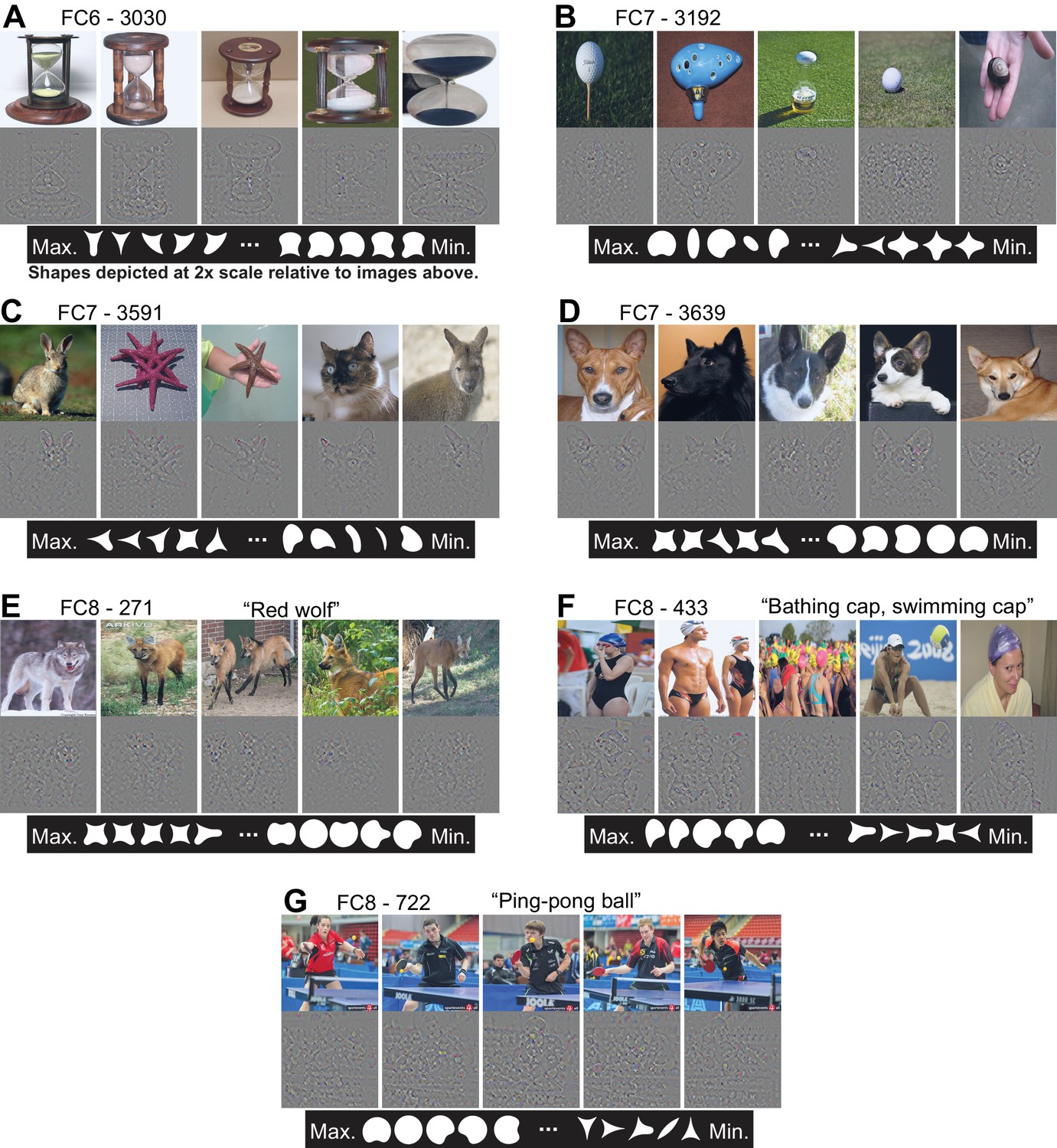
Visualization of APC-like units in the FC layers.
(A) For unit FC6-3030, the top five images from the test set are shown above their deconvolved feature maps. The maximal RF for all FC units includes the entire image. At bottom, the top five shapes are shown in order from left to right, followed by the bottom five shapes such that the shape associated with the minimum response is the rightmost. For visibility, shapes are shown here at twice the scale relative to the images. (B) For unit FC7-3192, same format as (A). (C) For unit FC7-3591, same format as (A). (D) For unit FC7-3639, same format as (A). (E) For unit FC8-271, same format as (A), except the category of this output-layer unit is indicated as 'Red wolf.’ (F) For unit FC8-433, same format as (E). (G) For unit FC8-722, same format as (E). See Table 1 for APC fit values for all units. Thumbnails featuring people were redacted for display in the published article, in line with journal policy. Input images were accessed via the ImageNet database and the original image URLs can be found through this site: http://image-net.org/about-overview.
© 2018, Various. Image thumbnails were taken from http://image-net.org and may be subject to copyright. They are not available under CC-BY and are exempt from the CC-BY 4.0 license.
Figure 13

Comparing the maximum responses driven by images to those driven by shapes for APC-like units.
For a given CNN unit, we computed the ratio of the maximum response across natural images (50,000 image test set) to the maximum response across our set of 362 shapes. The average of this ratio across the top ten APC-like units in each of seven layers (Conv2 to FC8) is plotted. Error bars show SD. In a few cases, the maximum response to shapes was a negative value and these cases were excluded: one unit for Conv3 and two for FC6 and FC7.
Figure 14
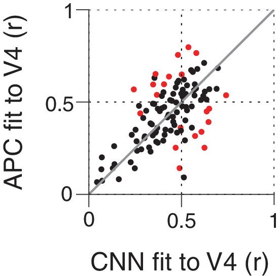
Comparing the ability of the APC model vs. single CNN units to fit V4 neuronal data.
Showing r-values for cross-validated fits from both classes of model, black points correspond to V4 neurons for which neither model performed significantly better at predicting responses to the shape set. The APC model provided a better fit for red points above the line of equality, whereas points below the line correspond to neurons for which at least one unit within the trained CNN provided a better fit than any APC model.
Tables
Table 1
Fit parameters and TI metric for example CNN units.
Unit numbers are given starting at zero in each sublayer. The APC model parameters, , , and , correspond to those in Equation 2. The TI metric is given by Equation 3. For visualization of preferred stimuli for example units, see Figures 9–12.
| Layer | Unit | APC r | TI | ||||
|---|---|---|---|---|---|---|---|
| Conv2 | 108 | 0.67 | 0.7 | 0.72 | 134 | 34 | 0.76 |
| Conv2 | 113 | 0.76 | 0.9 | 0.39 | 134 | 22 | 0.70 |
| Conv2 | 126 | 0.67 | 0.1 | 0.72 | 337 | 51 | 0.81 |
| Conv3 | 20 | 0.68 | 0.5 | 0.01 | 224 | 171 | 0.90 |
| Conv3 | 156 | 0.67 | 0.5 | 0.01 | 337 | 171 | 0.79 |
| Conv3 | 334 | 0.73 | 0.2 | 0.12 | 157 | 171 | 0.74 |
| Conv4 | 203 | 0.71 | 0.2 | 0.16 | 292 | 171 | 0.77 |
| Conv5 | 144 | 0.65 | 0.9 | 0.29 | 89 | 30 | 0.89 |
| Conv5 | 161 | 0.72 | 0.2 | 0.16 | 112 | 87 | 0.85 |
| FC6 | 3030 | 0.73 | −0.1 | 0.16 | 89 | 26 | 0.89 |
| FC7 | 3192 | 0.75 | 0.2 | 0.16 | 112 | 171 | 0.91 |
| FC7 | 3591 | 0.78 | −0.1 | 0.16 | 112 | 44 | 0.89 |
| FC7 | 3639 | 0.76 | −0.1 | 0.16 | 112 | 114 | 0.92 |
| FC8 | 271 | 0.73 | −0.1 | 0.16 | 112 | 114 | 0.91 |
| FC8 | 433 | 0.70 | 0.3 | 0.21 | 112 | 130 | 0.91 |
| FC8 | 722 | 0.72 | 0.2 | 0.08 | 112 | 130 | 0.93 |
Additional files
Download links
A two-part list of links to download the article, or parts of the article, in various formats.
Downloads (link to download the article as PDF)
Open citations (links to open the citations from this article in various online reference manager services)
Cite this article (links to download the citations from this article in formats compatible with various reference manager tools)
'Artiphysiology' reveals V4-like shape tuning in a deep network trained for image classification
eLife 7:e38242.
https://doi.org/10.7554/eLife.38242


