Step-to-step variations in human running reveal how humans run without falling
Figures
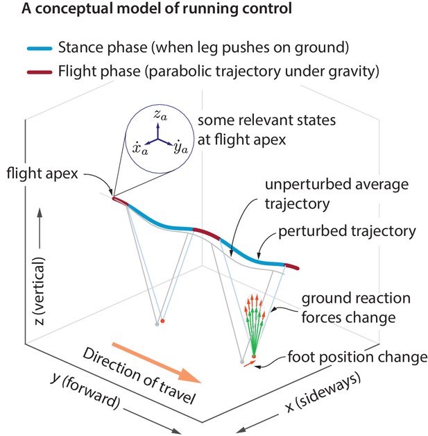
Idealized running control.
A schematic of a running trajectory, perturbed sideways during flight. The runner can recover back to steady state by changing the ground reaction force — say, by altering the foot placement and the leg force magnitude. This conceptual model is supported by our analysis of running data.
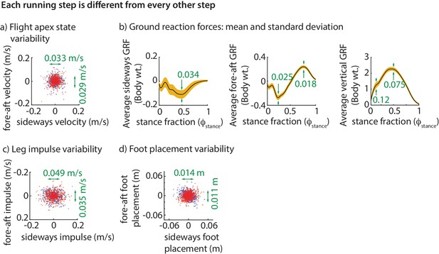
Step-to-step variability during running.
(a) Variability in the center of mass velocity at flight apex. (b) Mean GRFs in three directions (black line) and one standard deviation around the mean (yellow band) for a right stance phase; left stance phase GRF is similar in fore-aft and vertical directions, but the sideways GRF is negative of that for the right stance. Green text indicates standard deviation values in all panels. GRFs are in fraction of body weight. (c) Variability in the fore-aft and sideways impulses due to the GRFs. (d) Variability in foot position relative to torso at the beginning of stance phase. In panels a, c and d each dot corresponds to a separate step and the scatter plot is for all subjects with each subject’s mean value subtracted, so that only variability about the mean is shown for 500 randomly chosen steps. Red dots denote right steps and blue dots denote left steps.
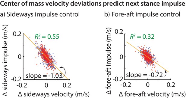
Center of mass velocity deviations predict stance impulse.
A linear model based on center of mass velocity deviations at flight apex explains a considerable fraction of the impulse on the next step. The impulses are mass-normalized. The scatter plot shows 500 randomly selected steps for left (blue dots) and right stances (red dots). The best-fit line (yellow) and the corresponding slope are shown for the left stance impulse. The slopes of the best fit line suggest that the sideways impulse corrects about 100% of the sideways velocity deviation on average and the fore-aft impulse corrects about 70% of the fore-aft velocity deviation.
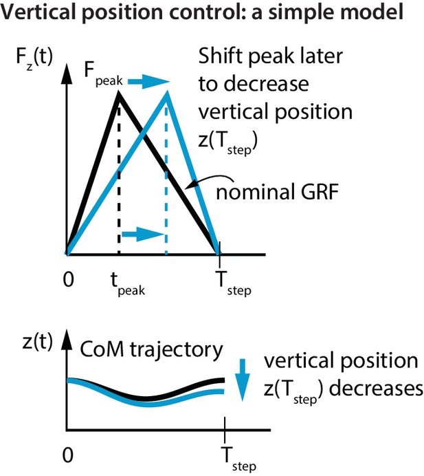
Vertical position control by differential impulse control.
Using a unimodal vertical GRF, we find that the way to lower vertical position over a step is to move the peak force to the right. This is equivalent to increasing the vertical impulse on the second half of the step and decreasing the vertical impulse over the first half. Conversely, to increase the vertical position over a step, we find that the peak force needs to be moved to the left.
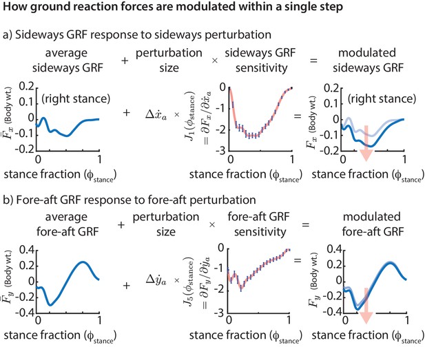
Phase-dependent control of GRFs.
We show how the GRF components respond to perturbations at the previous flight apex, as estimated by our phase-dependent GRF model. (a) Sideways GRF response to a (rightward) sideways velocity perturbation. (b) Fore-aft GRF response to a forward velocity perturbation. In both cases, the change in GRF from nominal (shown by the arrow) is obtained as a product of the perturbation size and the sensitivity of the GRF to the perturbation. To produce these plots, we computed a sequence of linear models, predicting the ground reaction forces at a sequence of gait phases through the stance phase, all using the same input variables, namely the flight apex center of mass state. The sensitivities or partial derivatives ( and ) shown are the corresponding coefficients in these linear models, plotted as a function of the stance fraction at which the GRF is being predicted by the linear model. In the axis labels, the nominal or average ground reaction forces are denoted with an overbar ( and ) and the modulated ground reaction forces are denoted without the overbar ( and ).
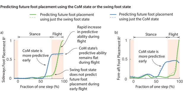
Swing foot control before foot placement.
The fraction of sideways foot placement (panel a) and fore-aft foot placement (panel b) variance at beginning of stance predicted by the center of mass (CoM) state or swing foot state during the previous one step (flight and stance). To produce this figure, a sequence of linear models were built for predicting the foot placement based on the center of mass state or swing foot state during different phases through the previous step. We plot the value corresponding to these linear models (that is, fraction of variance explained) as a function of the gait phase used for the prediction; the gait phase is represented as the fraction of a step starting from beginning of previous stance phase. The solid and dashed lines represent right and left foot placements, respectively.
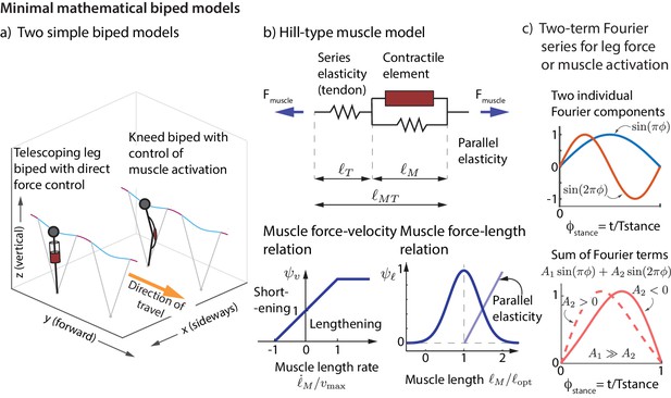
Minimal mathematical biped models.
(a) Two simple biped models were simulated: a telescoping leg model with direct force control and a kneed biped with activation control of the muscle at the knee. (b) The muscle in the second model is a classic Hill-type muscle (Zajac, 1989), composed of an active contractile element, a series elastic element (tendon), and a parallel elastic element. The force in the active contractile element for the muscle model depends on the muscle length through a force-length relationship , on the muscle length rate through a force-velocity relation , and the activation , so that , where is the maximum isometric force in the muscle (Zajac, 1989). (c) The control input for both models is represented as a Fourier sum of two sine waves of frequencies and . For the first model, the force is represented by this Fourier sum and for the second model, the muscle activation. This two-term function is able to allow leg force profiles without a time-reversal symmetry as shown (force peak not occurring at mid-stance).
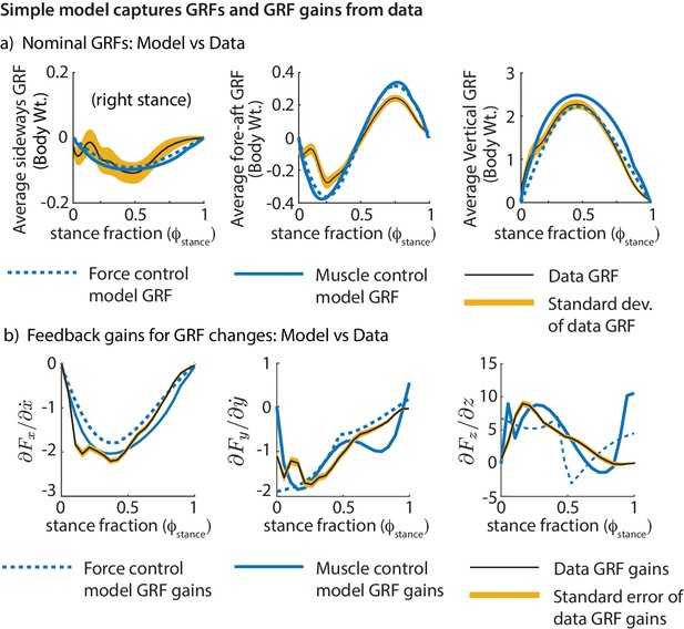
Comparing the simple biped models and human running data.
Both models fit the experimental GRFs and feedback gains reasonably well, despite not having been made to match them explicitly: (a) Mean GRFs over stance in three directions. GRFs are reported as a fraction of body weight. (b) Phase-dependent feedback gains describing the sensitivity of the sideways GRF to sideways velocity perturbation, fore-aft GRF to a fore-aft velocity perturbation, and the vertical GRF to vertical position perturbation at the previous flight apex. The standard deviations of the experimentally derived curves are shown as yellow bands.
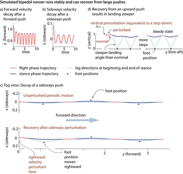
Stability of running in the simple biped model using the human-derived controller.
We illustrate the stability of the running model by showing how large perturbations at flight apex decay. (a) Decay of a forward velocity perturbation. (b) Decay of a sideways velocity perturbation. (c) Top view center of mass trajectory, showing the unperturbed running motion and a running motion that recovers from a rightward velocity perturbation. The rightward perturbation elicits a rightward foot placement, compared to the nominal foot placement during unperturbed running. (d) Sagittal view of running, recovering from an upward position perturbation. On the first step, the leg touch-down angle is steeper than the touch-down angle during unperturbed running and the contact time is shorter. All quantities are non-dimensional. See Videos 1,2 and 3 for illustrative animations of the biped model recovering from forward, sideways, and vertical perturbations, respectively.

Work loop and net leg work.
Work loops for the muscle-driven biped model without perturbations and with perturbations in the (a) fore-aft velocity, (b) sideways velocity, and (c) vertical position. The work loop plots force versus leg length and the signed area included in it is the net work performed by the leg.
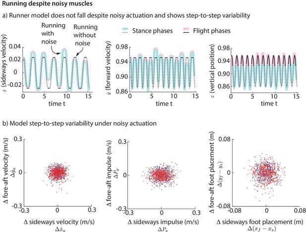
Running with noise.
(a) Multiple steps of the biped model running in the presence of noisy foot placement and muscle activations (blue for stance phases and pink for flight phases). Periodic nominal motion in the absence of noise (black, solid lines for stance, dashed for flight). (b) Deviations in flight apex state, GRF impulse, and foot placement from nominal for a 1000 steps (500 left steps as blue dots, 500 right steps as red dots), showing behavior analogous to Figure 2. This variability is not explicitly specified, but instead emerges from the interaction between the motor noise and the controlled dynamics.
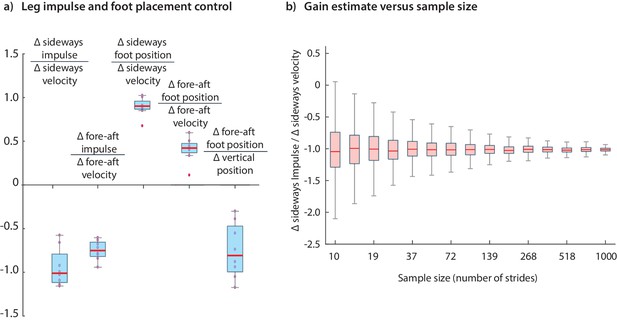
Variability in control gains due to subjects and sample sizes.
(a) The coefficients in the impulse control equations (Equations 1-2) and foot placement equations (Equations 8-9). The box plots indicate distributions of coefficients over all subjects; coefficients for each subject are also shown (red circles). (b) The dependence of coefficient estimate on the sample size, namely the number of strides used. The box plot indicates variability in control gain estimates. This plot was generated using bootstrap statistics (Efron and Tibshirani, 1994) by resampling from the pooled data from all subjects, and plotting the distribution of control gains obtained for each over multiple samples. This graph corresponds to the left stance impulses, but the corresponding graph for the right stances is nearly identical. Other coefficients exhibit similar trends with sample size. The boxes in the box plots show the median and the 25th to 75th percentile and the whiskers indicate all data within 2.7 standard deviations from the median.
Videos
Animation of point-mass biped model with the human-derived controller recovering from a forward velocity perturbation.
https://doi.org/10.7554/eLife.38371.012Animation of point-mass biped model with the human-derived controller recovering from a sideways velocity perturbation.
https://doi.org/10.7554/eLife.38371.013Animation of point-mass biped model with the human-derived controller recovering from a vertical position perturbation.
https://doi.org/10.7554/eLife.38371.014Additional files
-
Transparent reporting form
- https://doi.org/10.7554/eLife.38371.018


