Figures and data in Unsupervised discovery of temporal sequences in high-dimensional datasets, with applications to neuroscience

Figures
Tables
Additional files

12 figures, 3 tables and 1 additional file

Figures

Figure 1 with 1 supplement

Download asset Open asset

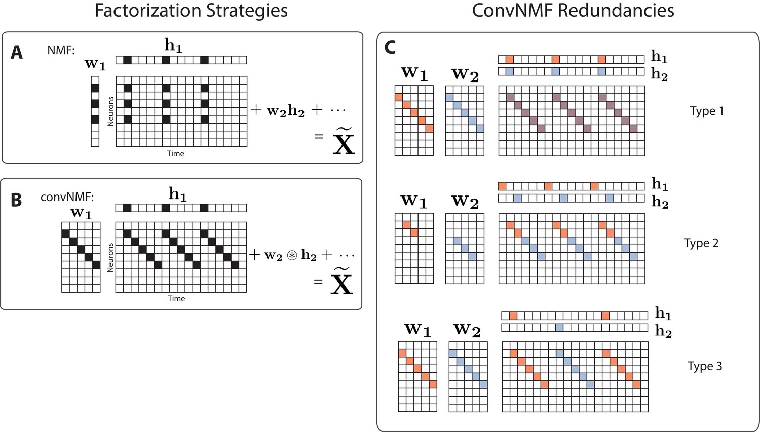
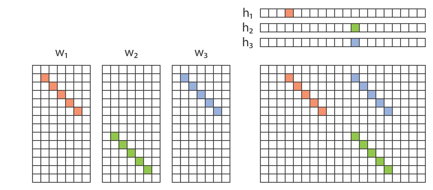
Convolutional NMF factorization.

(A) NMF (non-negative matrix factorization) approximates a data matrix describing the activity of $N$ neurons at $T$ timepoints as a sum of $K$ rank-one matrices. Each matrix is generated as the outer product of two nonnegative vectors: $𝐰_{k}$ of length $N$ , which stores a neural ensemble, and $𝐡_{k}$ of length $T$ , which holds the times at which the neural ensemble is active, and the relative amplitudes of this activity. (B) Convolutional NMF also approximates an $N \times T$ data matrix as a sum of $K$ matrices. Each matrix is generated as the convolution of two components: a non-negative matrix $𝐰_{k}$ of dimension $N \times L$ that stores a sequential pattern of the $N$ neurons at $L$ lags, and a vector of temporal loadings, $𝐡_{k}$ , which holds the times at which each factor pattern is active in the data, and the relative amplitudes of this activity. (C) Three types of inefficiencies present in unregularized convNMF: Type 1, in which two factors are used to reconstruct the same instance of a sequence; Type 2, in which two factors reconstruct a sequence in a piece-wise manner; and Type 3, in which two factors are used to reconstruct different instances of the same sequence. For each case, the factors ( $𝐖$ and $𝐇$ ) are shown, as well as the reconstruction ( $\tilde{𝐗} = 𝐖 ⊛ 𝐇 = 𝐰_{1} ⊛ 𝐡_{1} + 𝐰_{2} ⊛ 𝐡_{2} + \dots$ ).

https://doi.org/10.7554/eLife.38471.002

Figure 1—figure supplement 1

Download asset Open asset

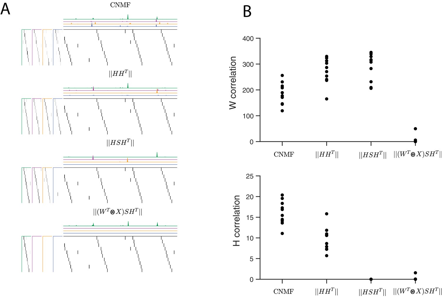
Quantifying the effect of different penalties on convNMF.

(A) Example factorizations of a synthetic dataset for convolutional NMF, and for convolutional NMF with three different penalties designed to eliminate correlations in $𝐇$ or in both $𝐇$ and $𝐖$ . Notice that different penalties lead to different types of redundancies in the corresponding factorizations. (B) Quantification of correlations in $𝐇$ and $𝐖$ for each different penalty. H correlations are measured using ${∥ {𝐇𝐒𝐇}^{⊤} ∥}_{1, i \neq j}$ and W correlations are measured using ${∥ 𝐖_{f l a t} 𝐖_{f l a t}^{⊤} ∥}_{1, i \neq j}$ , where $𝐖_{f l a t} = \sum_{ℓ} (𝐖_{\cdot, \cdot ℓ})$ .

https://doi.org/10.7554/eLife.38471.003

Figure 2 with 2 supplements

Download asset Open asset

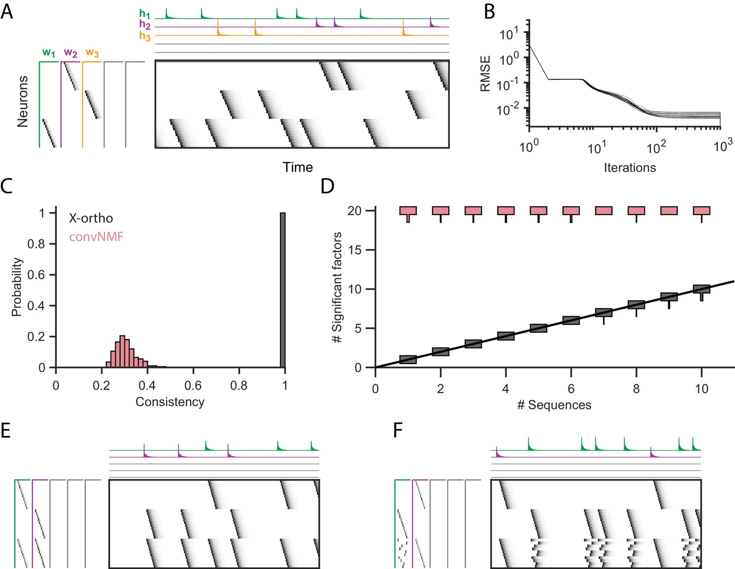
Effect of the x-ortho penalty on the factorization of sequences.

(A) A simulated dataset with three sequences. Also shown is a factorization with x-ortho penalty ( $K = 20$ , $L = 50$ , $λ = 0.003$ ). Each significant factor is shown in a different color. At left are the exemplar patterns ( $𝐖$ ) and on top are the timecourses ( $𝐇$ ). (B) Reconstruction error as a function of iteration number. Factorizations were run on a simulated dataset with three sequences and 15,000 timebins ( $\approx$ 60 instances of each sequence). Twenty independent runs are shown. Here, the algorithm converges to within 10% of the asymptotic error value within $\approx$ 100 iterations. (C) The x-ortho penalty produces more consistent factorizations than unregularized convNMF across 400 independent fits ( $K = 20$ , $L = 50$ , $λ = 0.003$ ). (D) The number of statistically significant factors (Figure 2—figure supplement 1) vs. the number of ground-truth sequences for factorizations with and without the x-ortho penalty. Shown for each condition is a vertical histogram representing the number of significant factors over 20 runs ( $K = 20$ , $L = 50$ , $λ = 0.003$ ). (E) Factorization with x-ortho penalty of two simulated neural sequences with shared neurons that participate at the same latency. (F) Same as E but for two simulated neural sequences with shared neurons that participate at different latencies.

https://doi.org/10.7554/eLife.38471.006

Figure 2—figure supplement 1

Download asset Open asset

Outline of the procedure used to assess factor significance.

(A) Distribution of overlap values between an extracted factor and the held-out data. (B) A null factor was constructed by randomly circularly shifting each row of a factor independently. Many null factors were constructed and the distribution of overlap values ( $𝐖 \overset{⊤}{⊛} 𝐗$ ) was measured between each null factor and the held-out data. (C) A comparison of the skewness values for each null factor and the skewness of the overlaps of the original extracted factor. A factor is deemed significant if its skewness is significantly greater than the distribution of skewness values for the null factor overlaps.

https://doi.org/10.7554/eLife.38471.007

Figure 2—figure supplement 2

Download asset Open asset

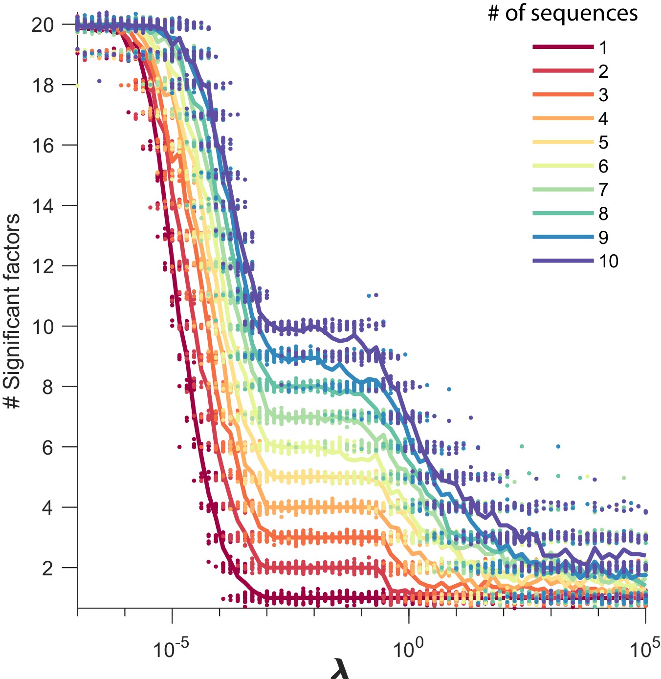
Number of significant factors as a function of $λ$ for datasets containing between 1 and 10 sequences.

The number of significant factors obtained by fitting data containing between 1 and 10 ground truth sequences using the x-ortho penalty ( $K = 20$ , $L = 50$ ) for a large range of values of $λ$ . For each value of $λ$ , 20 fits are shown and the mean is shown as a solid line. Each color corresponds to a ground-truth dataset containing a different number of sequences and no added noise. Values of $λ$ ranging between $0.001$ and $0.1$ tended to return the correct number of significant sequences at least 90% of the time.

https://doi.org/10.7554/eLife.38471.008

Figure 3 with 3 supplements

Download asset Open asset

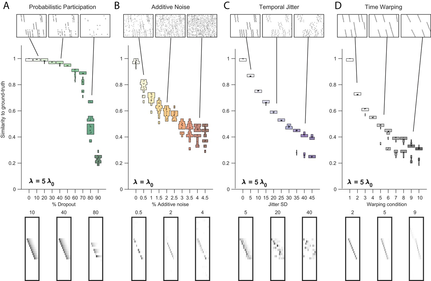
Testing factorization performance on sequences contaminated with noise.

Performance of the x-ortho penalty was tested under four different noise conditions: (A) probabilistic participation, (B) additive noise, (C) temporal jitter, and (D) sequence warping. For each noise type, we show: (top) examples of synthetic data at three different noise levels; (middle) similarity of extracted factors to ground-truth patterns across a range of noise levels (20 fits for each level); and (bottom) examples of extracted factors $𝐖$ ’s for one of the ground-truth patterns. Examples are shown at the same three noise levels illustrated in the top row. In these examples, the algorithm was run with $K = 20$ , $L = 50$ and $λ$ = $2 λ_{0}$ (via the procedure described in Figure 4). For C, jitter displacements were draw from a discrete guassian distribution with the standard deviation in timesteps shown above For D, timewarp conditions 1–10 indicate: 0, 66, 133, 200, 266, 333, 400, 466, 533 and 600 max % stretching respectively. For results at different values of $λ$ , see Figure 3—figure supplement 1.

https://doi.org/10.7554/eLife.38471.009

Figure 3—figure supplement 1

Download asset Open asset

Robustness to noise at different values of $λ$ .

Performance of the x-ortho penalty was tested under four different noise conditions, at different values of $λ$ than in Figure 3 (where $λ = 2 λ_{0}$ ): (A) probabilistic participation, $λ = 5 λ_{0}$ , (B) additive noise, $λ = λ_{0}$ (C) timing jitter, $λ = 5 λ_{0}$ and (D) sequence warping, $λ = 5 λ_{0}$ . For each noise type, we show: (top) examples of synthetic data at three different noise levels; (middle) similarity of x-ortho factors to ground-truth factors across a range of noise levels (20 fits for each level); and (bottom) example of one of the $𝐖$ ’s extracted at three different noise levels (same conditions as data shown above). The algorithm was run with $K = 20$ , $L = 50$ .

https://doi.org/10.7554/eLife.38471.010

Figure 3—figure supplement 2

Download asset Open asset

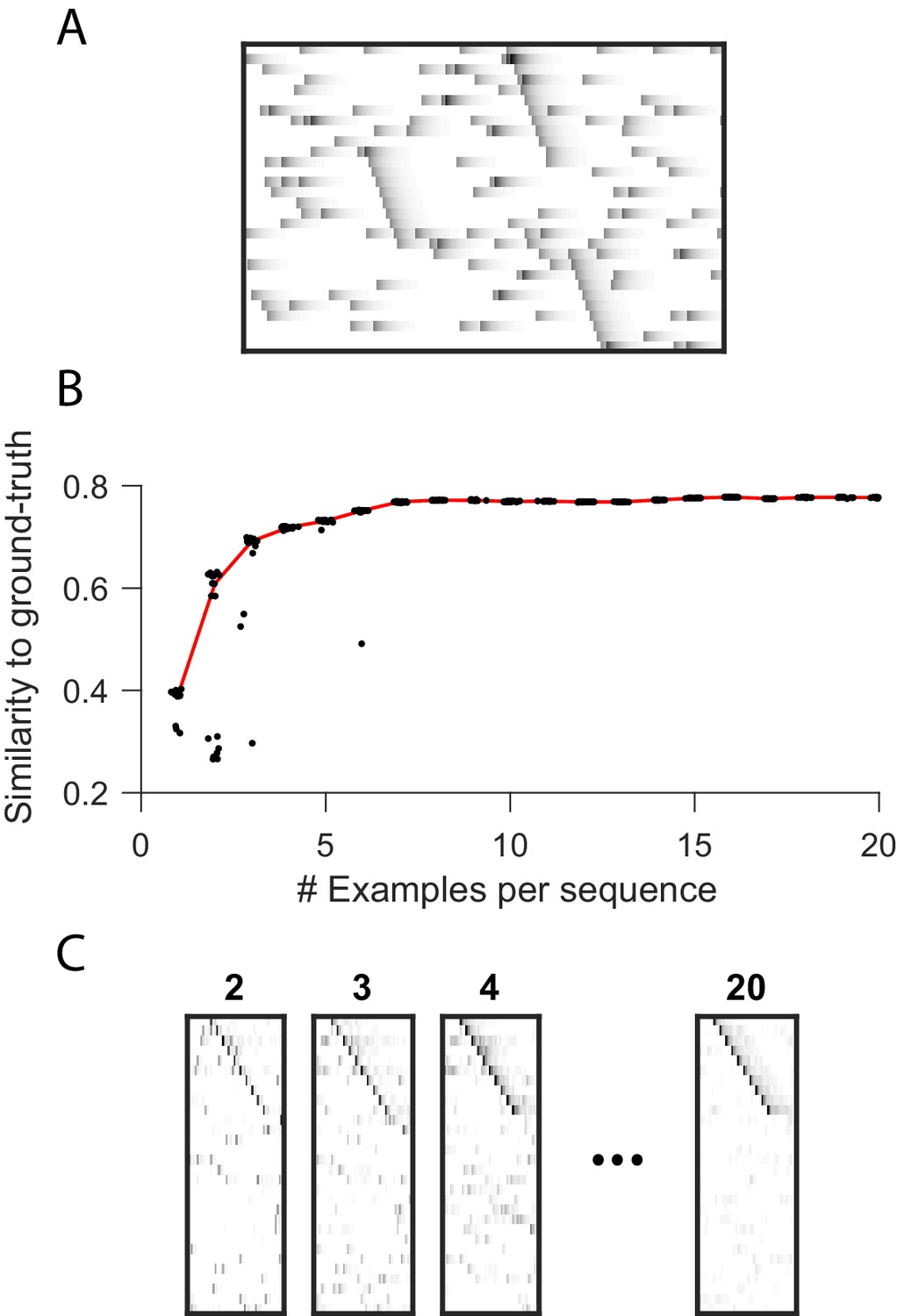
Robustness to small dataset size when using the x-ortho penalty.

(A) A short (400 timestep) dataset containing one example each of three ground-truth sequences, as well as additive noise. (B) As a function of dataset size, similarity of extracted factors to noiseless, ground-truth factors. At each dataset size, 20 independent fits of penalized convNMF are shown. Median shown in red. Three examples of each sequence were sufficient to acheive similiarty scores within 10% of asymptotic performance. (C) Example factors fit on data containing 2, 3, 4 or 20 examples of each sequence. Extracted factors were significant on held-out data compared to null (shuffled) factors even when training and test datasets each contained only 2 examples of each sequence.

https://doi.org/10.7554/eLife.38471.011

Figure 3—figure supplement 3

Download asset Open asset

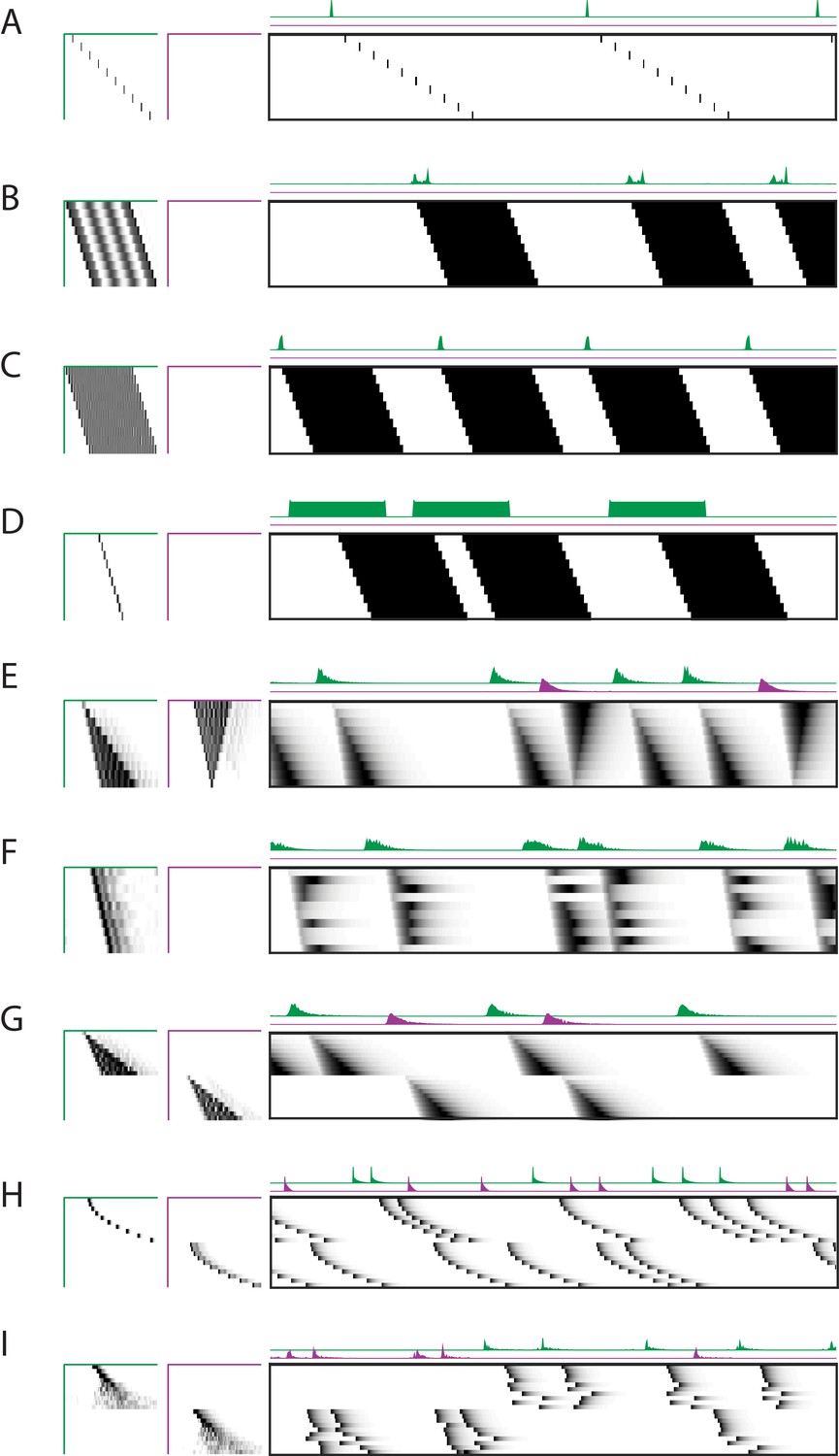
Robustness to different types of sequences.

Characterization of the x-ortho penalty for additional types of noise. (A) An example of a factorization for a sequence with large gaps between members of the sequence. (**B–D**) Example factorizations of sequences with neuronal activations that are highly overlapped in time. (B) An example of an x-ortho penalized factorization that reconstructs the data using complex patterns in $𝐖$ and $𝐇$ . (C) An example of an x-ortho penalized factorization with the addition of an L1 penalty on $𝐇$ models the data as an overlapping pattern with sparse activations. (D) An example of an x-ortho penalized factorization with the addition of an L1 penalty on $𝐖$ models the data as a non-overlapping pattern with dense activations. (E) An example of an x-ortho penalized factorization for data in which neurons have varying durations of activation which form two patterns. (F) An example of an x-ortho penalized factorization for data in which neurons have varying durations of activation which are random. (**G–I**) Examples factorizations of sequences with statistics that vary systematically. (G) An example of an x-ortho penalized factorization for data in which neurons have systematically varying changes in duration of activity. (H) An example of an x-ortho penalized factorization for data in which neurons have systematically varying changes in the gaps between members of the sequence. (I) An example of an x-ortho penalized factorization for data in which neurons have systematically varying changes in the amount of jitter.

https://doi.org/10.7554/eLife.38471.012

Figure 4 with 5 supplements

Download asset Open asset

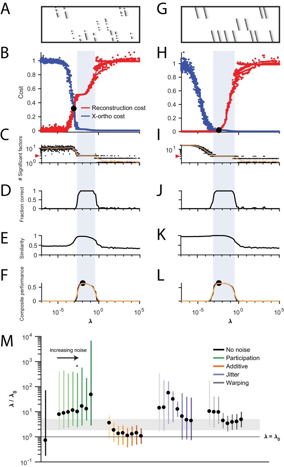
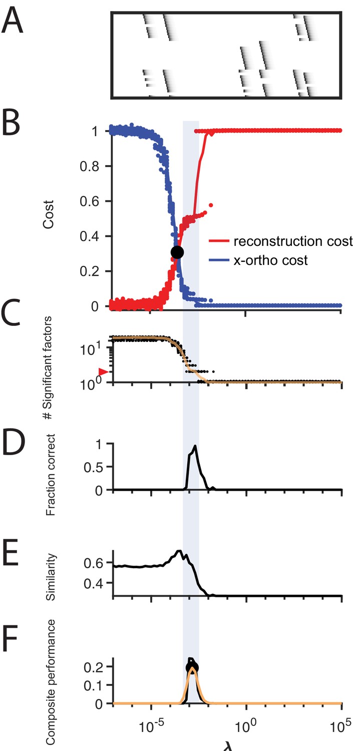
Procedure for choosing $λ$ for a new dataset based on finding a balance between reconstruction cost and x-ortho cost.

(A) Simulated data containing three sequences in the presence of participation noise (50% participation probability). This noise condition is used for the tests in (**B–F**). (B) Normalized reconstruction cost ( ${|| \tilde{𝐗} - 𝐗 ||}_{F}^{2}$ ) and cross-orthogonality cost ( ${|| (𝐖 \overset{⊤}{⊛} 𝐗) {𝐒𝐇}^{⊤} ||}_{1, i \neq j}$ ) as a function of $λ$ for 20 fits of these data. The cross-over point $λ_{0}$ is marked with a black circle. Note that in this plot the reconstruction cost and cross-orthogonality cost are normalized to vary between 0 and 1. (C) The number of significant factors obtained as a function of $λ$ ; 20 fits, mean plotted in orange. Red arrow at left indicates the correct number of sequences (three). (D) Fraction of fits returning the correct number of significant factors as a function of $λ$ . (E) Similarity of extracted factors to ground-truth sequences as a function of $λ$ . (F) Composite performance, as the product of the curves in (D) and (E) (smoothed using a three sample boxcar, plotted in orange with a circle marking the peak). Shaded region indicates the range of $λ$ that works well ( $\pm$ half height of composite performance). (**G–L**) same as (**A–F**) but for simulated data containing three noiseless sequences. (M) Summary plot showing the range of values of $λ$ (vertical bars), relative to the cross-over point $λ_{0}$ , that work well for each noise condition ( $\pm$ half height points of composite performance). Circles indicate the value of $λ$ at the peak of the smoothed composite performance. For each noise type, results for all noise levels from Figure 3 are shown (increasing color saturation at high noise levels; Green, participation: 90, 80, 70, 60, 50, 40, 30, and 20%; Orange, additive noise 0.5, 1, 2, 2.5, 3, 3.5, and 4%; Purple, jitter: SD of the distribution of random jitter: 5, 10, 15, 20, 25, 30, 35, 40, and 45 timesteps; Grey, timewarp: 66, 133, 200, 266, 333, 400, 466, 533, 600, and 666 max % stretching. Asterisk (*) indicates the noise type and level used in panels (**A–F**). Gray band indicates a range between $2 λ_{0}$ and $5 λ_{0}$ , a range that tended to perform well across the different noise conditions. In real data, it may be useful to explore a wider range of $λ$ .

https://doi.org/10.7554/eLife.38471.013

Figure 4—figure supplement 1

Download asset Open asset

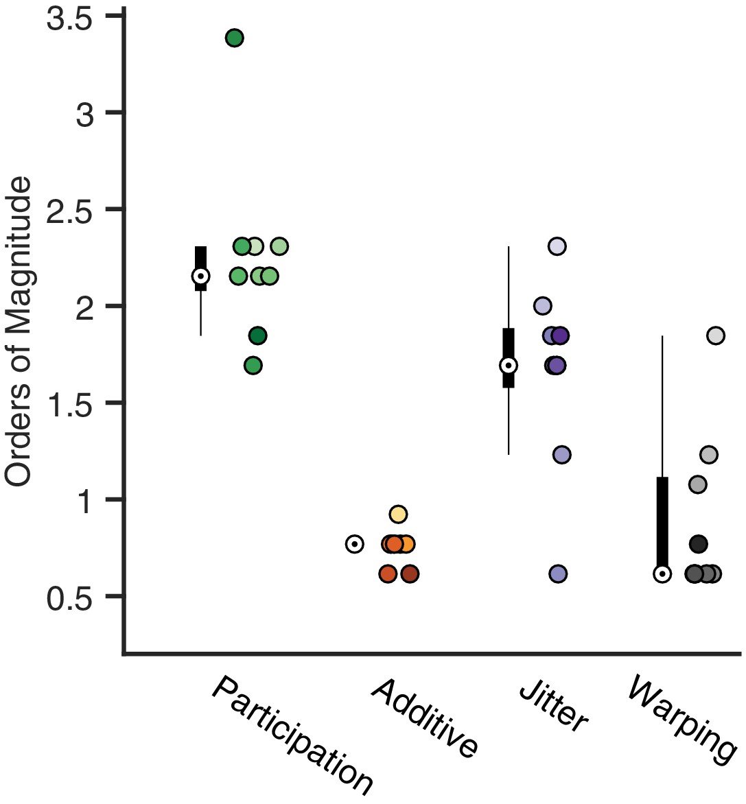
Analysis of the best range of $λ$ .

Here, we quantify the full width at the half maximum for the composite performance scores in different noise conditions. For each condition, a box and whisker plot quantifies the number of orders of magnitude over which a good factorization is returned (median denoted by a white circle). Next to each box plot individual points are shown, corresponding to different noise level. Color saturation reflects noise level as in Figure 4.

https://doi.org/10.7554/eLife.38471.014

Figure 4—figure supplement 2

Download asset Open asset

Procedure for choosing $λ$ applied to data with shared neurons.

(A) Simulated data containing two patterns which share 50% of their neurons, in the presence of participation noise (70% participation probability). (B) Normalized reconstruction cost ( ${|| \tilde{𝐗} - 𝐗 ||}_{F}^{2}$ ) and cross-orthogonality cost ( ${|| (𝐖 \overset{⊤}{⊛} 𝐗) {𝐒𝐇}^{⊤} ||}_{1, i \neq j}$ ) as a function of $λ$ for these data. The cross-over point $λ_{0}$ is marked with a black circle. (C) The number of significant factors obtained from 20 fits of these data as a function of $λ$ (mean number plotted in orange). The correct number of factors (two) is marked by a red triangle. (D) The fraction of fits returning the correct number of significant factors as a function of $λ$ . (E) Similarity of the top two factors to ground-truth (noiseless) factors as a function of $λ$ . (F) Composite performance measured as the product of the curves shown in (D) and (E), (smoothed curve plotted in orange with a circle marking the peak). Shaded region indicates the range of $λ$ that works well ( $\pm$ half height of composite performance). For this dataset, the best performance occurs at $λ = 5 λ_{0}$ , while a range of $λ$ between 2 $λ_{0}$ and 10 $λ_{0}$ performs well.

https://doi.org/10.7554/eLife.38471.015

Figure 4—figure supplement 3

Download asset Open asset

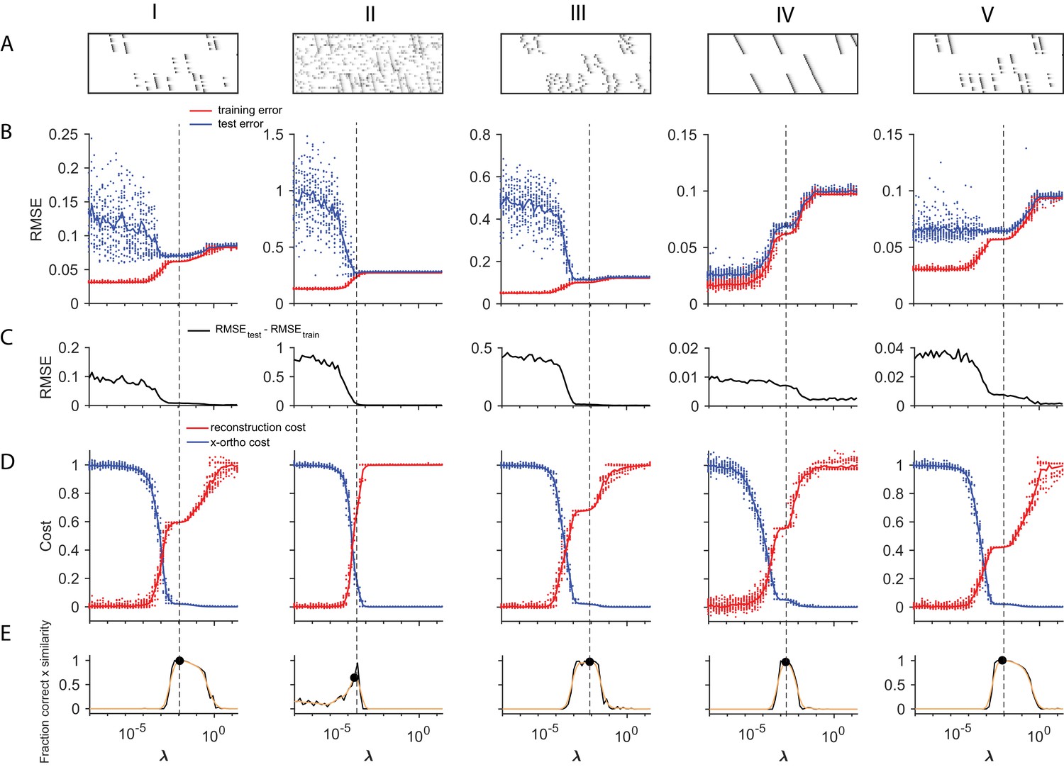
Using cross-validation on held-out (masked) data to choose $λ$ .

A method for choosing a reasonable value of $λ$ based on cross validation is shown for five different noise types (each column shows a different noise type; from left to right: (I) participation noise, (II) additive noise, (III) jitter, (IV) temporal warping), and (V) a lower level of participation noise. The cross-validated test error is calculated by fitting x-ortho penalized factorizations while randomly holding out 10% of the elements in the data matrix as a test set (Wold, 1978; Bro et al., 2008). In many of our test datasets, there was a minimum or a divergence point in the difference between the test and training error, that agreed with the procedure described in Figure 4, based on $λ_{0}$ . (A) Examples of each dataset. (B) Test error (blue) and training error (red) as a function of $λ$ for each of the different noise conditions. (C) The difference between the test error and training error values shown above. (D) Normalized reconstruction cost ( ${|| \tilde{𝐗} - 𝐗 ||}_{F}^{2}$ ) and cross-orthogonality cost ( ${|| (𝐖 \overset{⊤}{⊛} 𝐗) {𝐒𝐇}^{⊤} ||}_{1, i \neq j}$ ) as a function of $λ$ for each of the different noise conditions. (E) Composite performance as a function of $λ$ . Panels D and E are identical to those in Figure 4, and are included here for comparison. (V) These data have a lower amount of participation noise than (I). Note that in low-noise conditions, test error may not exhibit a minima within the range of $λ$ that produces the ground truth number of factors.

https://doi.org/10.7554/eLife.38471.016

Figure 4—figure supplement 4

Download asset Open asset

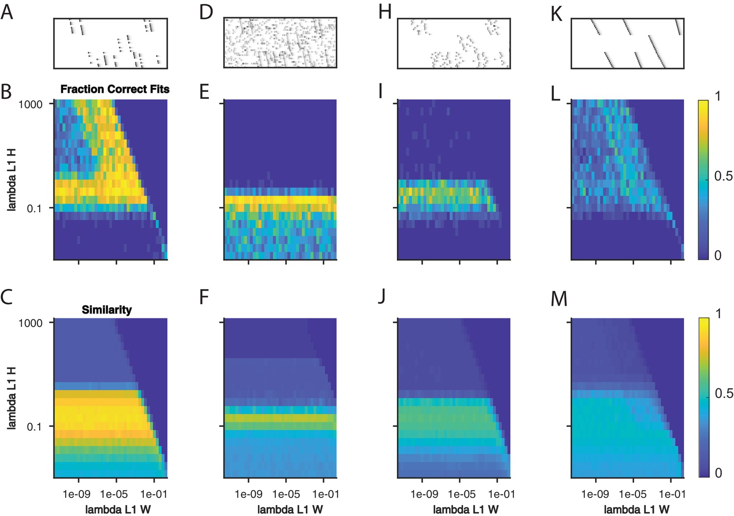
Quantifying the effect of L1 sparsity penalties on $𝐖$ and $𝐇$ .

(A) An example window of simulated data with three sequences and 40% dropout. (B) The fraction of fits to data with the noise level in (A) that yielded three significant factors, as a function of two L1 sparsity regularization parameters on $𝐖$ and $𝐇$ . Each bin represents 20 fits of sparsity penalized convNMF with K = 20 and L = 50. (C) The mean similarity to ground-truth for the same 20 factorizations as in (B). (**D–F**) same as panels A-C but with additional noise events in 2.5% of the bins. (**H–J**) same as panels A-C but with a jitter standard deviation of 20 bins. (**K–M**) same as panels A-C but for warping noise with a maximum of 260% warping.

https://doi.org/10.7554/eLife.38471.017

Figure 4—figure supplement 5

Download asset Open asset

Comparing the performance of convNMF with an x-ortho or a sparsity penalty.

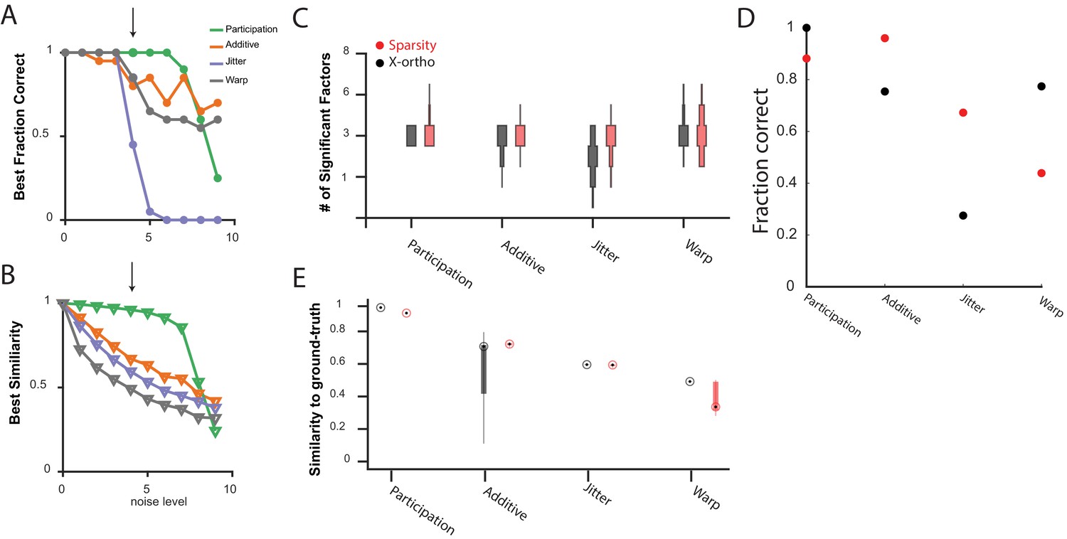
(A) The fraction of 20 x-ortho penalized fits which had the same number of significant factors as the ground-truth for all noise conditions shown in Figure 3 at the $λ$ with the best performance. (B) The similarity to ground-truth for 20 x-ortho penalized fits to all noise conditions shown in Figure 3 at the $λ$ with the best performance. (C) The number of significant factors for 100 fits with an x-ortho penalty (black) and with sparsity penalties on $𝐖$ and $𝐇$ (Red) of four different noise conditions at the level indicated in (A) and (B). Penalty parameters used in (**C–E**) were selected by performing a parameter sweep and selecting the parameters which gave the maximum composite score as described above. (D) The fraction of 20 x-ortho or sparsity penalized fits with the ground truth number of significant sequences. Noise conditions are the same as in (C). Values for $λ$ were selected as those that give the highest composite performance (see Figure 4F). (E) Similarity to ground-truth for the fits shown in (**C–D**). Median is shown with black dot and bottom and top edges of boxes indicate the 25^th and 75^th percentiles.

https://doi.org/10.7554/eLife.38471.018

Figure 5 with 2 supplements

Download asset Open asset

Direct selection of K using the *diss* metric, a measure of the dissimilarity between different factorizations.

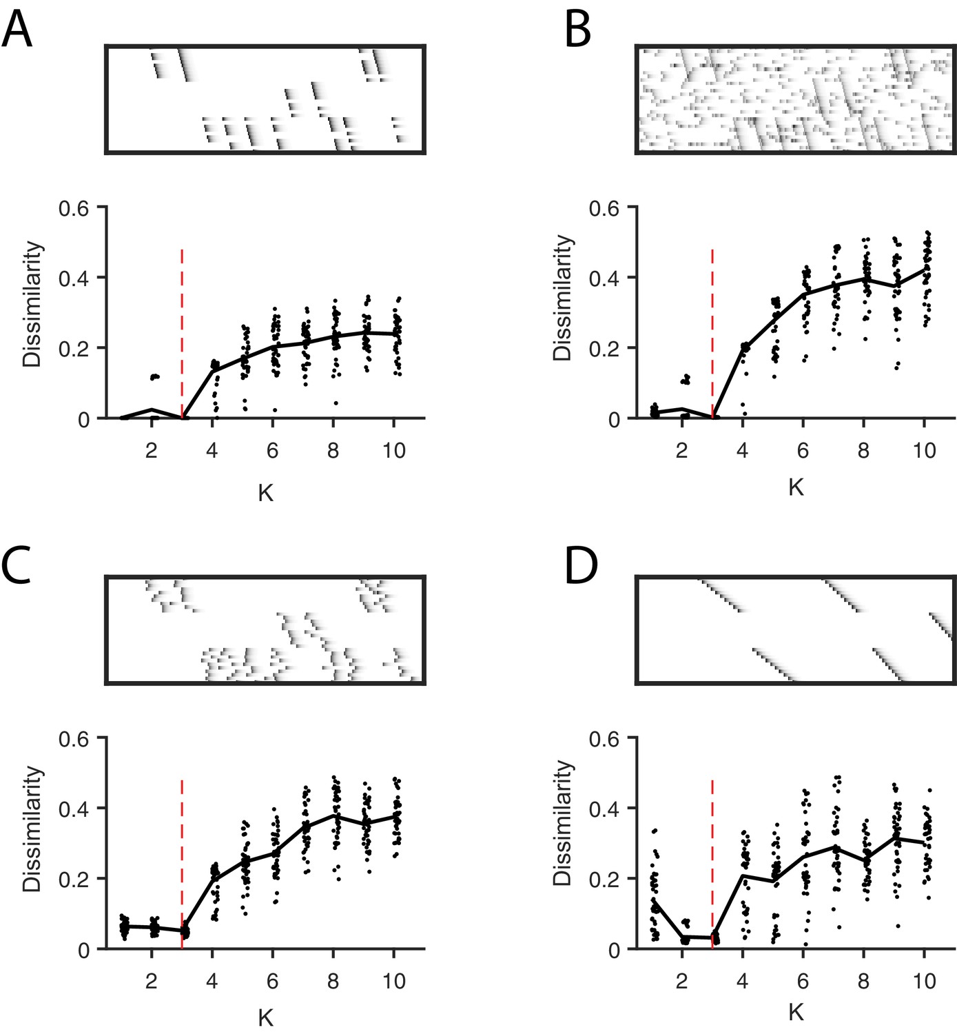
Panels show the distribution of *diss* as a function of K for several different noise conditions. Lower values of *diss* indicate greater consistency or stability of the factorizations, an indication of low factor redundancy. (A) probabilistic participation (60%), (B) additive noise (2.5% bins), (C) timing jitter (SD = 20 bins), and (D) sequence warping (max warping = 266%). For each noise type, we show: (top) examples of synthetic data; (bottom) the *diss* metric for 20 fits of convNMF for K from 1 to 10; the black line shows the median of the *diss* metric and the dotted red line shows the true number of factors.

https://doi.org/10.7554/eLife.38471.019

Figure 5—figure supplement 1

Download asset Open asset

Direct selection of K using the *diss* metric for all noise conditions.

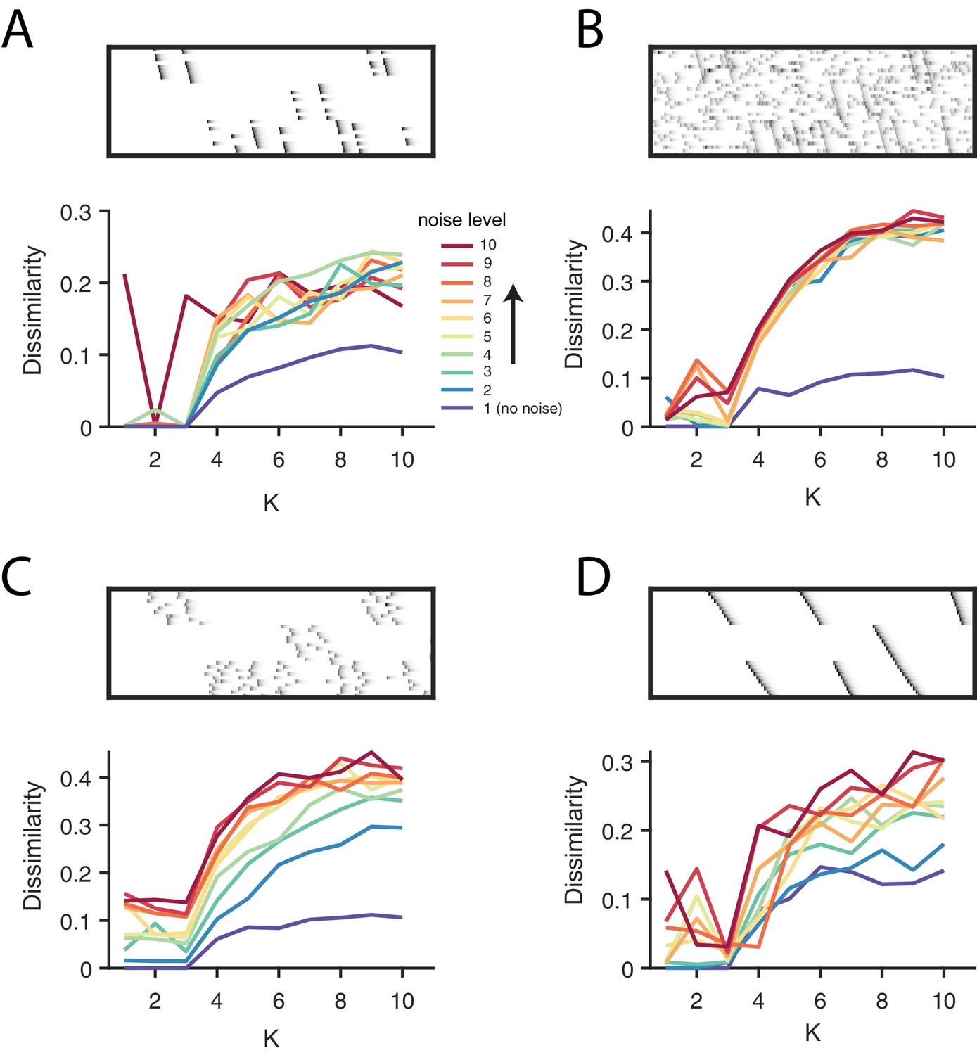
(A) Participation noise, (B) additive noise, (C) jitter and (D) warping. For each panel, the top shows an example of data with three sequences and each noise type. The bottom panel shows the dissimilarity of factorizations in different levels of noise, as a function of K. A condition with no noise is shown in blue and dark red represents the highest noise condition with the color gradient spanning the levels between. Noise levels are the same as in Figure 3 and Figure 4. Notice that there is often either a minimum or a distinct feature at K = 3, corresponding to the ground-truth number of sequences in the data.

https://doi.org/10.7554/eLife.38471.020

Figure 5—figure supplement 2

Download asset Open asset

Estimating the number of sequences in a dataset using cross-validation on randomly masked held-out datapoints.

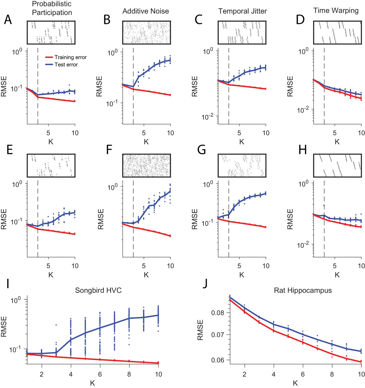
(A) Reconstruction error (RMSE) for test data (red) and training data (blue) plotted as a function of the number of components (K) used in convNMF. Twenty independent convNMF fits are shown for each value of K. This panel shows results for 10% participation noise. For synthetic data fits, 10% of the data was held out as the test set. For neural data 5% of the data was held out. Other noise conditions are shown as follows: (B) jitter noise (10 timestep SD); (C) warping (13%); (D) higher additive noise (2.5%); (E) higher jitter noise (25 timestep SD); (F) higher warping (33%) (G) Reconstruction error vs. K for neuronal data collected from premotor cortex (area HVC) of a singing bird (Figure 9) and (H) hippocampus of rat 2 performing a left-right alternation task (Figure 8).

https://doi.org/10.7554/eLife.38471.021

Figure 6 with 1 supplement

Download asset Open asset

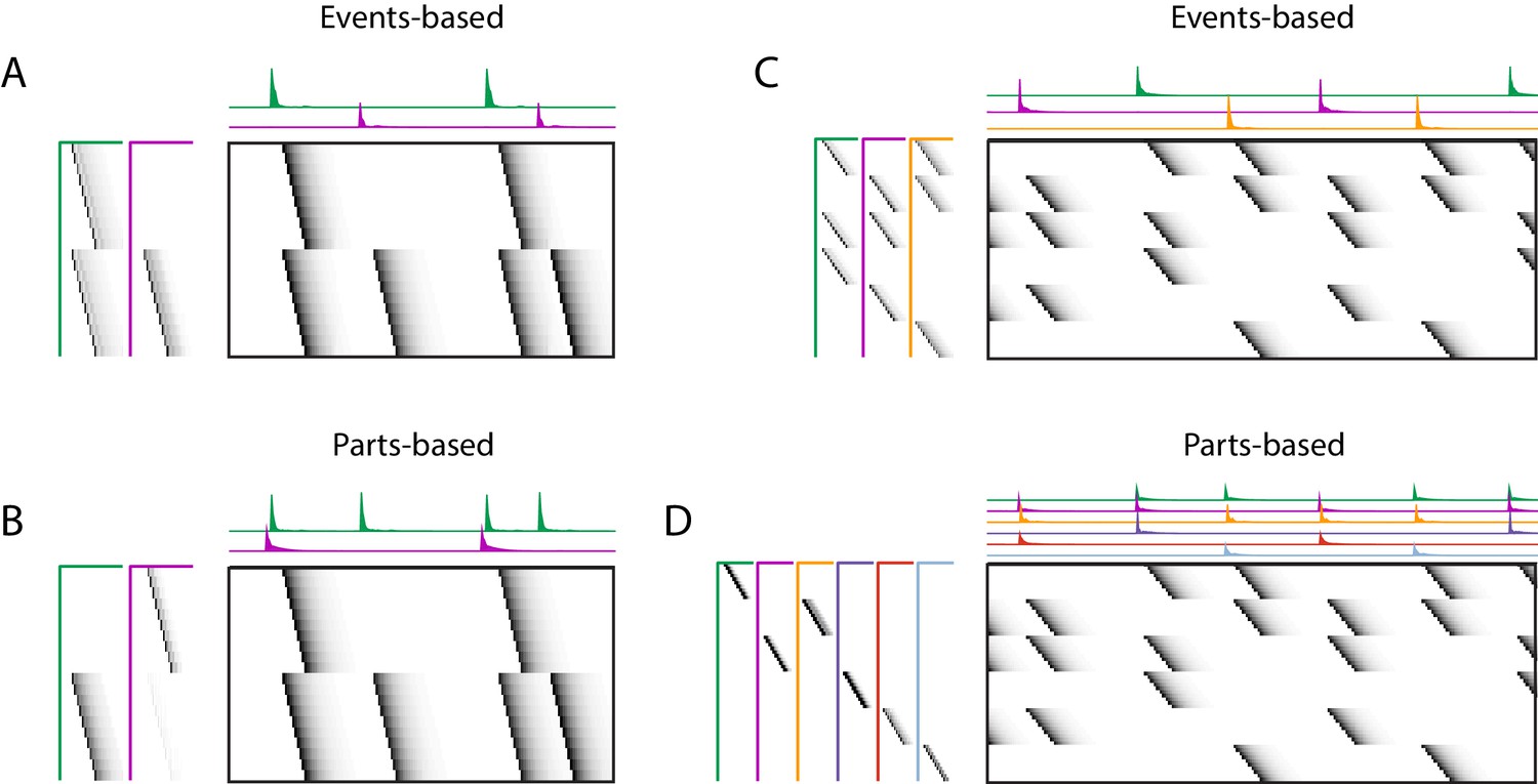
Using penalties to bias toward events-based and parts-based factorizations.

Datasets that have neurons shared between multiple sequences can be factorized in different ways, emphasizing discrete temporal events (events-based) or component neuronal ensembles (parts-based), by using orthogonality penalties on $𝐇$ or $𝐖$ to penalize factor correlations (see Table 2). (Left) A dataset with two different ensembles of neurons that participate in two different types of events, with (A) events-based factorization obtained using an orthogonality penalty on $𝐇$ and (B) parts-based factorizations obtained using an orthogonality penalty on $𝐖$ . (Right) A dataset with six different ensembles of neurons that participate in three different types of events, with (C) events-based and (D) parts-based factorizations obtained as in (A) and (B).

https://doi.org/10.7554/eLife.38471.022

Figure 6—figure supplement 1

Download asset Open asset

Biasing factorizations between sparsity in $𝐖$ or $𝐇$ .

Two different factorizations of the same simulated data, where a sequence is always repeated precisely three times. Both yield perfect reconstructions, and no cross-factor correlations. The factorizations differ in the amount of features placed in $𝐖$ versus $𝐇$ . Both use $K = 3$ and $λ = 0.001$ . (A) Factorization achieved using a sparsity penalty on $𝐇$ , with $λ_{L 1 𝐇} = 1$ . (B) Factorization achieved using a sparsity penalty on $𝐖$ , with $λ_{L 1 𝐖} = 1$ .

https://doi.org/10.7554/eLife.38471.023

Figure 7

Download asset Open asset

Using seqNMF to assess the prevalence of sequences in noisy data.

(A) Example simulated datasets. Each dataset contains 10 neurons, with varying amounts of additive noise, and varying proportions of synchronous events versus asynchronous sequences. For the purposes of this figure, 'sequence' refers to a sequential pattern with no synchrony between different neurons in the pattern. The duration of each dataset used below is 3000 times, and here 300 timebins are shown. (B) Median percent power explained by convNMF (L = 12; K = 2; $λ$ =0) for each type of dataset (100 examples of each dataset type). Different colors indicate the three different levels of additive noise shown in A. Solid lines and filled circles indicate results on unshuffled datasets. Note that performance is flat for each noise level, regardless of the probability of sequences vs synchronous events. Dotted lines and open circles indicate results on column-shuffled datasets. When no sequences are present, convNMF performs the same on column-shuffled data. However, when sequences are present, convNMF performs worse on column-shuffled data. (C) For datasets with patterns ranging from exclusively synchronous events to exclusively asynchronous sequences, convNMF was used to generate a ‘Sequenciness’ score. Colors correspond to different noise levels shown in A. Asterisks denote cases where the power explained exceeds the Bonferroni-corrected significance threshold generated from column-shuffled datasets. Open circles denote cases that do not achieve significance. Note that this significance test is fairly sensitive, detecting even relatively low presence of sequences, and that the ‘Sequenciness’ score distinguishes between cases where more or less of the dataset consists of sequences.

https://doi.org/10.7554/eLife.38471.024

Figure 8

Download asset Open asset

Application of seqNMF to extract hippocampal sequences from two rats.

(A) Firing rates of 110 neurons recorded in the hippocampus of Rat 1 during an alternating left-right task with a delay period (Pastalkova et al., 2015). The single significant extracted x-ortho penalized factor. Both an x-ortho penalized reconstruction of each factor (left) and raw data (right) are shown. Neurons are sorted according to the latency of their peak activation within the factor. The red line shows the onset and offset of the forced delay periods, during which the animal ran on a treadmill. (B) Firing rates of 43 hippocampal neurons recorded in Rat 2 during the same task (Mizuseki et al., 2013). Neurons are sorted according to the latency of their peak activation within each of the three significant extracted sequences. The first two factors correspond to left and right trials, and the third corresponds to running along the stem of the maze. (C) The *diss* metric as a function of K for Rat 1. Black line represents the median of the black points. Notice the minimum at K = 1. (D) (Left) Reconstruction (red) and correlation (blue) costs as a function of $λ$ for Rat 1. Arrow indicates $λ = 8 \times 10^{- 5}$ , used for the x-ortho penalized factorization shown in (A). (E) Histogram of the number of significant factors across 30 runs of x-ortho penalized convNMF. (D) The *diss* metric as a function of K for Rat 2. Notice the minimum at K = 3. (**G–H**) Same as in (**D–E**) but for Rat 2. Arrow indicates $λ = 8 \times 10^{- 5}$ , used for the factorization shown in (B).

https://doi.org/10.7554/eLife.38471.025

Figure 9 with 2 supplements

Download asset Open asset

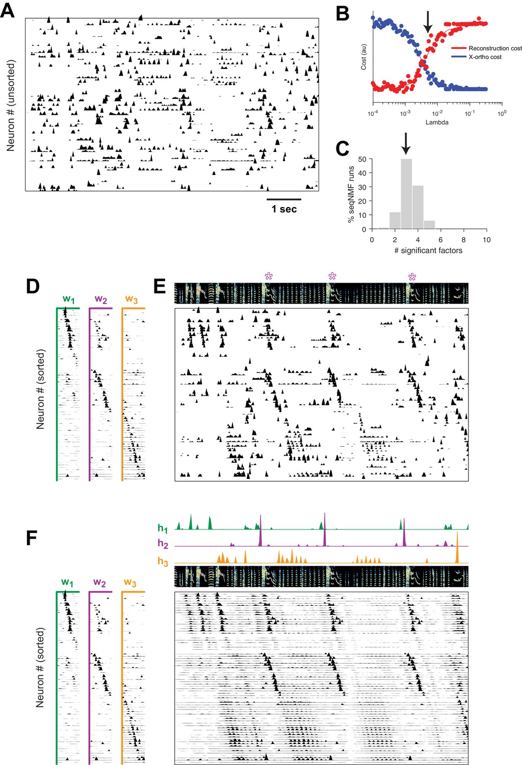
SeqNMF applied to calcium imaging data from a singing isolate bird reveals abnormal sequence deployment.

(A) Functional calcium signals recorded from 75 neurons, unsorted, in a singing isolate bird. (B) Reconstruction and cross-orthogonality cost as a function of $λ$ . The arrow at $λ = 0.005$ indicates the value selected for the rest of the analysis. (C) Number of significant factors for 100 runs with the x-ortho penalty with $K = 10$ , $λ = 0.005$ . Arrow indicates three is the most common number of significant factors. (D) X-ortho factor exemplars ( $𝐖$ ’s). Neurons are grouped according to the factor in which they have peak activation, and within each group neurons are sorted by the latency of their peak activation within the factor. (E) The same data shown in (A), after sorting neurons by their latency within each factor as in (D). A spectrogram of the bird’s song is shown at top, with a purple ‘*’ denoting syllable variants correlated with $𝐰_{2}$ . (F) Same as (E), but showing reconstructed data rather than calcium signals. Shown at top are the temporal loadings ( $𝐇$ ) of each factor.

https://doi.org/10.7554/eLife.38471.026

Figure 9—figure supplement 1

Download asset Open asset

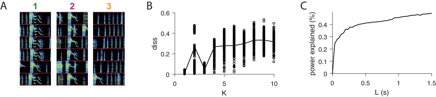
Further analysis of sequences.

(A) For each of the three extracted sequences, examples of song spectrograms triggered at moments where there is a peak in H. Different examples are separated by a red line. Note that each sequence factor corresponds to a particular syllable type. (B) As a function of $K$ , *diss* measure across all combinations of 10 fits of convNMF. Note the local minima at K = 3. (C) Percent power explained (for convNMF with K = 3 and $λ = 0$ ) as a function of L. Note the bend that truncates at approximately 0.25 s, corresponding to a typical syllable duration.

https://doi.org/10.7554/eLife.38471.027

Figure 9—figure supplement 2

Download asset Open asset

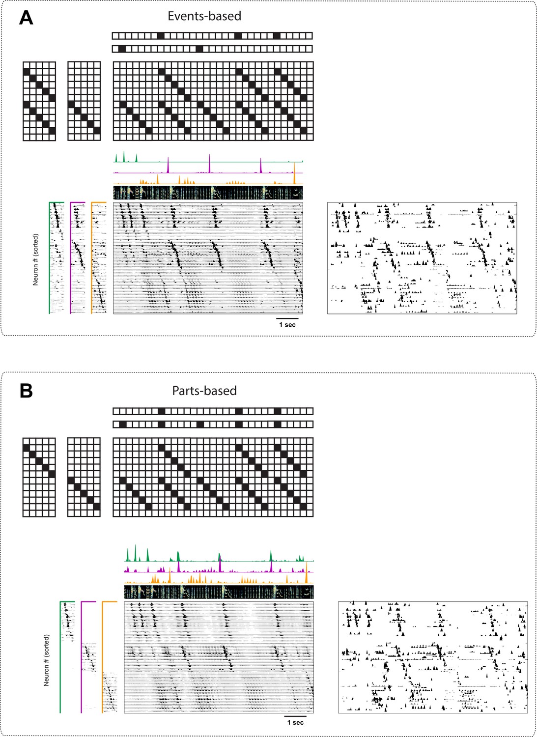
Events-based and parts-based factorizations of songbird data.

Illustration of a trade-off between parts-based ( $𝐖$ is more strictly orthogonal) and events-based ( $𝐇$ is more strictly orthogonal) factorizations in a dataset where some neurons are shared between different sequences. The same data as in Figure 9 is factorized with an orthogonality cost just on $𝐇$ (A, events-based), or just on $𝐖$ (B, parts-based). Below each motivating cartoon factorization, we show x-ortho penalized convNMF fits ( $𝐖$ and $𝐇$ together with the reconstruction) of the data in Figure 9. The right panels contain the raw data sorted according to these factorizations. Favoring events-based or parts-based factorizations is a matter of preference. Parts-based factorizations are particularly useful for separating neurons into ensembles. Events-based factorizations are particularly useful for identifying what neural events occur when.

https://doi.org/10.7554/eLife.38471.028

Figure 10

Download asset Open asset

SeqNMF applied to song spectrograms.

(A) Spectrogram of juvenile song, with hand-labeled syllable types (Okubo et al., 2015). (B) Reconstruction cost and x-ortho cost for these data as a function of $λ$ . Arrow denotes $λ = 0.0003$ , which was used to run convNMF with the x-ortho penalty (C) $𝐖$ ’s for this song, fit with $K = 8$ , $L = 200 m s$ , $λ = 0.0003$ . Note that there are three non-empty factors, corresponding to the three hand-labeled syllables a, b, and c. (D) X-ortho penalized $𝐇$ ’s (for the three non-empty factors) and reconstruction of the song shown in (A) using these factors.

https://doi.org/10.7554/eLife.38471.029

Appendix 2—figure 1

Download asset Open asset

Example of redundancy with three factors.

In addition to the direct overlap of $𝐡_{2}$ and $𝐡_{3}$ , and of $𝐰_{1}$ and $𝐰_{3}$ , there is a ‘triplet’ penalty $𝐑_{12}$ on factors 1 and 2 that occurs because each has an overlap (in either $𝐖$ or $𝐇$ ) with the 3rd factor ( $𝐰_{3}, 𝐡_{3}$ ). This occurs even though neither $𝐰_{1}$ and $𝐰_{2}$ , nor $𝐡_{1}$ and $𝐡_{2}$ , are themselves overlapping.

https://doi.org/10.7554/eLife.38471.034

Author response image 1

Download asset Open asset

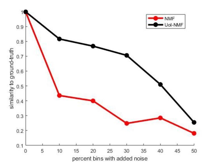
Validation of our adaptations of UoI-NMF.

Similarity to ground-truth as a function of additive noise level for UoI-NMF factorizations and NMF factorizations using the algorithmic changes detailed above.

Note that UoI-NMF extracts bases which are closer to the ground-truth patterns than regular NMF.

https://doi.org/10.7554/eLife.38471.036

Tables

Table 1

Notation for convolutional matrix factorization

https://doi.org/10.7554/eLife.38471.004

Shift operator

The operator

\overset{ℓ \to}{(H)}

shifts a matrix

𝐇

in the

\to

direction by

ℓ

timebins:

{\overset{ℓ \to}{(H)}}_{\cdot t} = H_{\cdot (t - l)}

and likewise

{\overset{\leftarrow ℓ}{(H)}}_{\cdot t} = H_{\cdot (t + ℓ)}

where

\cdot

indicates all elements along the respective matrix dimension.

The shift operator inserts zeros when

(t - ℓ) < 0

(t + ℓ) > T

Tensor convolution operator

Convolutive matrix factorization reconstructs a data matrix

𝐗

using a

N \times K \times L

tensor

𝐖

and a

K \times T

matrix

𝐇

\tilde{𝐗} = 𝐖 ⊛ 𝐇 = \sum_{ℓ} 𝐖_{\cdot, \cdot ℓ} \overset{ℓ \to}{𝐇}

Note that each neuron

n

is reconstructed as the sum of

k

convolutions:

{\tilde{𝐗}}_{n t} = \sum_{k} \sum_{ℓ} 𝐖_{n k ℓ} 𝐇_{k (t - ℓ)} \equiv {(𝐖 ⊛ 𝐇)}_{n t}

Transpose tensor convolution operator

The following quantity is useful in several contexts:

𝐖 \overset{⊤}{⊛} 𝐗 = \sum_{ℓ} {(𝐖_{\cdot, \cdot ℓ})}^{⊤} \overset{\leftarrow ℓ}{𝐗}

Note that each element

{(𝐖 \overset{⊤}{⊛} 𝐗)}_{k t} = \sum_{l} {(𝐖_{\cdot k ℓ})}^{⊤} 𝐗_{\cdot (t + ℓ)} = \sum_{l} \sum_{n} 𝐖_{n k ℓ} 𝐗_{n (t + ℓ)}

measures

the overlap (correlation) of factor

k

with the data at time

t

convNMF reconstruction

𝐗 \approx \tilde{𝐗} = \sum_{k} 𝐖_{\cdot k, \cdot} ⊛ 𝐇_{k, \cdot} = 𝐖 ⊛ 𝐇

Note that NMF is a special case of convNMF, where

L = 1

L 1

entrywise norm excluding diagonal elements

For any

K \times K

matrix

𝐂

{∥ 𝐂 ∥}_{1, i \neq j} \equiv \sum_{k} \sum_{j \neq k} 𝐂_{j k}

Special matrices

𝟏

is a

K \times K

matrix of ones

𝐈

is the

K \times K

identity matrix

𝐒

is a

T \times T

smoothing matrix:

𝐒_{i j} = 1

when

| i - j | < L

and otherwise

𝐒_{i j} = 0

Table 2

Regularized NMF and convNMF: cost functions and algorithms

https://doi.org/10.7554/eLife.38471.005

NMF
$ℒ = \frac{1}{2} {\|\| \tilde{𝐗} - 𝐗 \|\|}_{2}^{2} + ℛ$ $\tilde{𝐗} = 𝐖𝐇$	$W \leftarrow W \times \frac{X H^{⊤}}{\tilde{X} H^{⊤} + \frac{\partial ℛ}{\partial W}}$ $H \leftarrow H \times \frac{W^{⊤} X}{W^{⊤} \tilde{X} + \frac{\partial ℛ}{\partial H}}$
convNMF
$ℒ = \frac{1}{2} {\|\| \tilde{𝐗} - 𝐗 \|\|}_{2}^{2} + ℛ$ $\tilde{𝐗} = 𝐖 ⊛ 𝐇$	$W_{\cdot \cdot ℓ} \leftarrow W_{\cdot \cdot ℓ} \times \frac{X {\overset{ℓ \to}{H}}^{⊤}}{\tilde{X} {\overset{ℓ \to}{H}}^{⊤} + \frac{\partial ℛ}{\partial W_{\cdot \cdot ℓ}}}$ $H \leftarrow H \times \frac{W \overset{⊤}{⊛} X}{W \overset{⊤}{⊛} \tilde{X} + \frac{\partial ℛ}{\partial H}}$
$L 1$ regularization for $𝐇$ ( $L 1$ for $𝐖$ is analogous)
$ℛ = λ {\|\| 𝐇 \|\|}_{1}$	$\frac{\partial ℛ}{\partial 𝐖_{\cdot, \cdot ℓ}} = 0$ $\frac{\partial ℛ}{\partial 𝐇} = λ 𝟏$
Orthogonality cost for $𝐇$
$ℛ = \frac{λ}{2} {\|\| {𝐇𝐇}^{⊤} \|\|}_{1, i \neq j}$	$\frac{\partial ℛ}{\partial 𝐖_{\cdot, \cdot ℓ}} = 0$ $\frac{\partial ℛ}{\partial 𝐇} = λ (𝟏 - 𝐈) 𝐇$
Smoothed orthogonality cost for $𝐇$ (favors ‘events-based’)
$ℛ = \frac{λ}{2} {\|\| {𝐇𝐒𝐇}^{⊤} \|\|}_{1, i \neq j}$	$\frac{\partial ℛ}{\partial 𝐖_{\cdot, \cdot ℓ}} = 0$ $\frac{\partial ℛ}{\partial 𝐇} = λ (𝟏 - 𝐈) 𝐇𝐒$
Smoothed orthogonality cost for $𝐖$ (favors ‘parts-based’)
$ℛ = \frac{λ}{2} {\|\| 𝐖_{f l a t}^{⊤} 𝐖_{f l a t} \|\|}_{1, i \neq j}$ where ${(𝐖_{f l a t})}_{n k} = \sum_{ℓ} 𝐖_{n k ℓ}$	$\frac{\partial ℛ}{\partial 𝐖_{\cdot, \cdot ℓ}} = λ 𝐖_{f l a t} (𝟏 - 𝐈)$ $\frac{\partial ℛ}{\partial 𝐇} = 0$
Smoothed cross-factor orthogonality (x-ortho penalty)
$ℛ = λ {\|\| (𝐖 \overset{⊤}{⊛} 𝐗) {𝐒𝐇}^{⊤} \|\|}_{1, i \neq j}$	$\frac{\partial ℛ}{\partial 𝐖_{\cdot, \cdot ℓ}} = λ \overset{\leftarrow ℓ}{𝐗} {𝐒𝐇}^{⊤} (𝟏 - 𝐈)$ $\frac{\partial ℛ}{\partial 𝐇} = λ (𝟏 - 𝐈) 𝐖 \overset{⊤}{⊛} 𝐗𝐒$

Key resources table

Reagent type (species) or resource	Designation	Source or reference	Identifiers	Additional information
Software, algorithm	seqNMF	this paper	https://github.com/FeeLab/seqNMF	start with demo.m
Software, algorithm	convNMF	Smaragdis, 2004; Smaragdis, 2007	https://github.com/colinvaz/nmf-toolbox
Software, algorithm	sparse convNMF	O’Grady and Pearlmutter, 2006; Ramanarayanan et al., 2013	https://github.com/colinvaz/nmf-toolbox
Software, algorithm	NMF orthogonality penalties	Choi, 2008; Chen and Cichocki, 2004
Software, algorithm	other NMF extensions	Cichocki et al., 2009
Software, algorithm	NMF	Lee and Seung, 1999
Software, algorithm	CNMF_E (cell extraction)	Zhou et al., 2018	https://github.com/zhoupc/CNMF_E
Software, algorithm	MATLAB	MathWorks	www.mathworks.com, RRID:SCR_001622
Strain, strain background (adeno-associated virus)	AAV9.CAG.GCaMP6f. WPRE.SV40	Chen et al., 2013	Addgene viral prep # 100836-AAV9, http://n2t.net/addgene:100836, RRID:Addgene_100836
Commercial assay or kit	Miniature microscope	Inscopix	https://www.inscopix.com/nvista

Additional files

Transparent reporting form: https://doi.org/10.7554/eLife.38471.031
Download elife-38471-transrepform-v2.pdf

Download links

A two-part list of links to download the article, or parts of the article, in various formats.

Downloads (link to download the article as PDF)

Open citations (links to open the citations from this article in various online reference manager services)

Mendeley

Cite this article (links to download the citations from this article in formats compatible with various reference manager tools)

Emily L Mackevicius
Andrew H Bahle
Alex H Williams
Shijie Gu
Natalia I Denisenko
Mark S Goldman
Michale S Fee

(2019)

Unsupervised discovery of temporal sequences in high-dimensional datasets, with applications to neuroscience

eLife 8:e38471.

https://doi.org/10.7554/eLife.38471

Figures

Convolutional NMF factorization.

Quantifying the effect of different penalties on convNMF.

Effect of the x-ortho penalty on the factorization of sequences.

Outline of the procedure used to assess factor significance.

Number of significant factors as a function of $λ$ for datasets containing between 1 and 10 sequences.

Testing factorization performance on sequences contaminated with noise.

Robustness to noise at different values of $λ$ .

Robustness to small dataset size when using the x-ortho penalty.

Robustness to different types of sequences.

Procedure for choosing $λ$ for a new dataset based on finding a balance between reconstruction cost and x-ortho cost.

Analysis of the best range of $λ$ .

Procedure for choosing $λ$ applied to data with shared neurons.

Using cross-validation on held-out (masked) data to choose $λ$ .

Quantifying the effect of L1 sparsity penalties on $𝐖$ and $𝐇$ .

Comparing the performance of convNMF with an x-ortho or a sparsity penalty.

Direct selection of K using the diss metric, a measure of the dissimilarity between different factorizations.

Direct selection of K using the diss metric for all noise conditions.

Estimating the number of sequences in a dataset using cross-validation on randomly masked held-out datapoints.

Using penalties to bias toward events-based and parts-based factorizations.

Biasing factorizations between sparsity in $𝐖$ or $𝐇$ .

Using seqNMF to assess the prevalence of sequences in noisy data.

Application of seqNMF to extract hippocampal sequences from two rats.

SeqNMF applied to calcium imaging data from a singing isolate bird reveals abnormal sequence deployment.

Further analysis of sequences.

Events-based and parts-based factorizations of songbird data.

SeqNMF applied to song spectrograms.

Example of redundancy with three factors.

Validation of our adaptations of UoI-NMF.

Tables

Notation for convolutional matrix factorization

Regularized NMF and convNMF: cost functions and algorithms

Additional files

Transparent reporting form

Download links

Downloads (link to download the article as PDF)

Open citations (links to open the citations from this article in various online reference manager services)

Cite this article (links to download the citations from this article in formats compatible with various reference manager tools)

Be the first to read new articles from eLife

Share this article

Cite this article

Convolutional NMF factorization.

Quantifying the effect of different penalties on convNMF.

Effect of the x-ortho penalty on the factorization of sequences.

Outline of the procedure used to assess factor significance.

Number of significant factors as a function of λ for datasets containing between 1 and 10 sequences.

Testing factorization performance on sequences contaminated with noise.

Robustness to noise at different values of λ.

Robustness to small dataset size when using the x-ortho penalty.

Robustness to different types of sequences.

Procedure for choosing λ for a new dataset based on finding a balance between reconstruction cost and x-ortho cost.

Analysis of the best range of λ.

Procedure for choosing λ applied to data with shared neurons.

Using cross-validation on held-out (masked) data to choose λ.

Quantifying the effect of L1 sparsity penalties on 𝐖 and 𝐇.

Comparing the performance of convNMF with an x-ortho or a sparsity penalty.

Direct selection of K using the diss metric, a measure of the dissimilarity between different factorizations.

Direct selection of K using the diss metric for all noise conditions.

Estimating the number of sequences in a dataset using cross-validation on randomly masked held-out datapoints.

Using penalties to bias toward events-based and parts-based factorizations.

Biasing factorizations between sparsity in 𝐖 or 𝐇.

Using seqNMF to assess the prevalence of sequences in noisy data.

Application of seqNMF to extract hippocampal sequences from two rats.

SeqNMF applied to calcium imaging data from a singing isolate bird reveals abnormal sequence deployment.

Further analysis of sequences.

Events-based and parts-based factorizations of songbird data.

SeqNMF applied to song spectrograms.

Example of redundancy with three factors.

Validation of our adaptations of UoI-NMF.

Notation for convolutional matrix factorization

Regularized NMF and convNMF: cost functions and algorithms

Transparent reporting form

Downloads (link to download the article as PDF)

Open citations (links to open the citations from this article in various online reference manager services)

Cite this article (links to download the citations from this article in formats compatible with various reference manager tools)

Number of significant factors as a function of $λ$ for datasets containing between 1 and 10 sequences.

Robustness to noise at different values of $λ$ .

Procedure for choosing $λ$ for a new dataset based on finding a balance between reconstruction cost and x-ortho cost.

Analysis of the best range of $λ$ .

Procedure for choosing $λ$ applied to data with shared neurons.

Using cross-validation on held-out (masked) data to choose $λ$ .

Quantifying the effect of L1 sparsity penalties on $𝐖$ and $𝐇$ .

Biasing factorizations between sparsity in $𝐖$ or $𝐇$ .