Control of entropy in neural models of environmental state
- University of Oxford, John Radcliffe Hospital, United Kingdom
- Radboud University, The Netherlands
- University College London, United Kingdom
- University of Oxford, United Kingdom
Figures
Figure 1 with 4 supplements
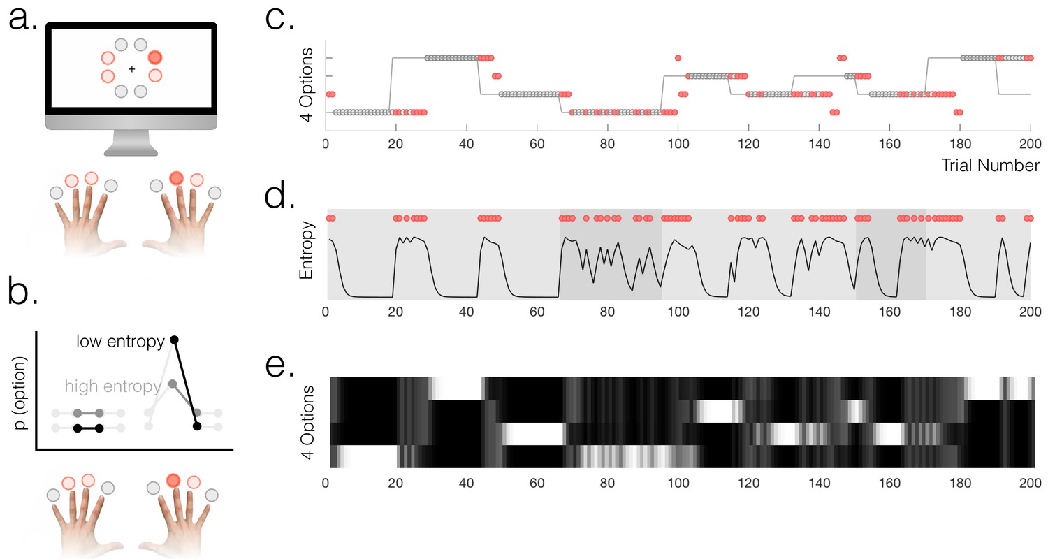
Task and behaviour.
(a) Participants chose freely between four available options on each trial. A total of 8 options were used in the experiment but only four were used in each run of the task (indicated by option colours: red circles above the fingers denote the available options, and the dark red circle denotes the selected option). (b) Schematic of a probabilistic model of the state of the environment – the weighting of each option represents its probability of being the high reward option. When entropy is low, i.e. participants are certain, the weighting of the selected option is higher than when entropy is high. (c) Example behaviour of a participant. Dot markers denote choices (location in y-dimension indicates which option was chosen) – grey circles are rewarded and red dots are unrewarded trials. The grey line indicates the true state of the world (high reward option), which the participant must infer. Note alternating phases of exploration and exploitation – the main analyses presented in the paper refer only to the exploitation phase in which there are no overt changes of action. (d) Model entropy for the same run as in (c). Note that model entropy is low during exploit periods but increases following a reward omission (red dots are trials with reward omission). Background shading indicates the pay-out rate of the high reward option: during low pay-out (70%) exploit periods, indicated in dark grey, entropy tends to remain higher; during high pay-out periods (light grey) entropy reaches a floor during exploitation. (e) State space of the model – four horizontal tracks represent the four possible states of the environment; shading indicates the posterior probability assigned to each state by the model (light colours indicate high probability).
Figure 1—figure supplement 1

Implementation of the task described in the Main Text and Methods.
Participants controlled a mouse seeking cheese or apples, counterbalanced across participants. Participants could select any of four available locations, denoted in this case by blue circles, again counterbalanced across participants. Please see the Main Text and Methods for details of the task.
Figure 1—figure supplement 2
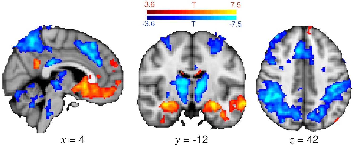
Exploitation and exploration engage different brain regions.
T-statistic map for the [1 -1] contrast in GLM1. Positive activation (hotter colours) denotes regions more active during exploitation than exploration, and vice versa for negative activation. Medial OFC and hippocampus were more active during exploitation, and a frontal-parietal action network was more active during exploration. Image thresholded at p<0.001; corrected for multiple comparisons using cluster mass-based permutation testing: cluster forming threshold is voxelwise p<0.001, cluster corrected threshold p<0.05.
Figure 1—figure supplement 3
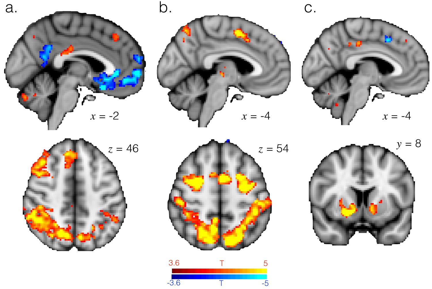
Activation related to task factors.
T-statistic maps for the entropy (a), whether changing response (b) and reward (c) regressors in GLM2. These variables explain variance in very similar brain regions to those in which variance is explained by differences between exploitation and exploration. Panels a and b images thresholded at p<0.001 and corrected for multiple comparisons. Panel c image thresholded at p<0.001, uncorrected.
Figure 1—figure supplement 4
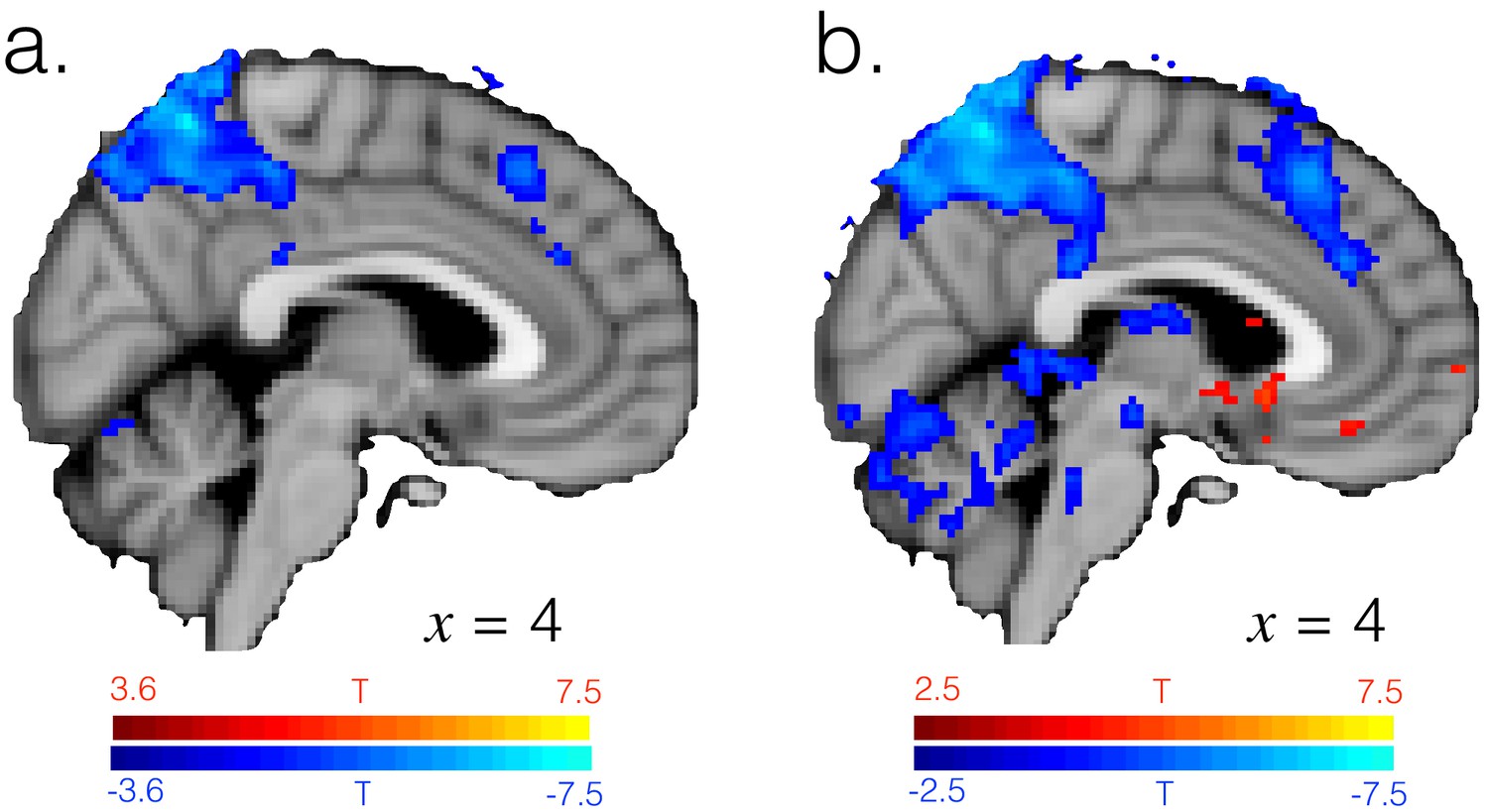
A large amount of the difference between exploitation and exploration is captured by task factors.
T-statistic map for the [1 -1] contrast in GLM3, testing for differences between exploitation and exploration having regressed out effects of the task factors. (a) Image thresholded voxelwise at p<0.001, the same threshold as in Figure 1—figure supplement 2, uncorrected. (b) Image thresholded voxelwise at a more liberal threshold of p<0.01, uncorrected.
Figure 2 with 2 supplements
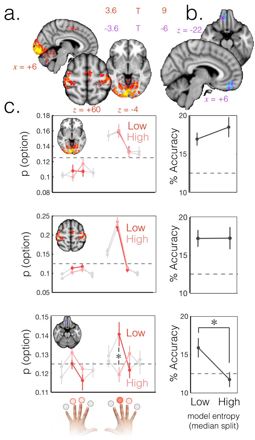
Probabilistic beliefs represented in mOFC.
(a) The currently selected option can be decoded above chance, as expected, in motor and visual cortex (t score map for above chance decoding of the chosen option across subjects; thresholded at p<0.001; corrected for multiple comparisons). (b) Medial OFC represents the current state of the task probabilistically. Highlighted voxels are the centers of searchlights in which the representation strength for the chosen option was higher when model entropy was low (i.e. when participants have high certainty about the state of the environment; t score map for the effect of model entropy on representation strength; thresholded at p<0.001; corrected for multiple comparisons). (c) Region of interest analyses demonstrating multivariate decoding patterns. Left column: the multivariate classifier probability that each option was selected; on trials when model entropy was low (dark red) and high (light red). Right column: decoding accuracy (i.e. proportion of trials when the option with the highest probability of having been selected by the classifier was indeed the option selected by the participant) in low and high entropy trials. All error bars are SEM. Dashed lines denote chance. Top row and middle row: decoding in visual and motor cortices, respectively, is not sensitive to model entropy and errors in decoding tend to be to neighbouring options. Bottom row: decoding in mOFC is modulated by model entropy, such that decoding is higher when model entropy is low.
Figure 2—figure supplement 1
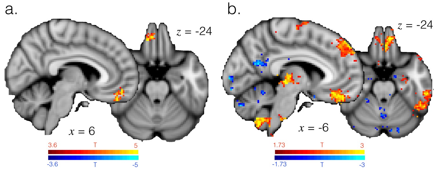
Representation strength in mOFC is explained by probability assigned to the currently selected option, as well as the difference between high and low reward exploit periods.
(a) T-statistic map showing model probability explains representation strength specifically in mOFC, as in GLM5. Image thresholded at p<0.001; corrected for multiple comparisons. (b) T-statistic map showing regions where representation strength is higher in high (90%) vs. low (70%) reward exploit periods. Image thresholded voxelwise at p<0.05, uncorrected.
Figure 2—figure supplement 2
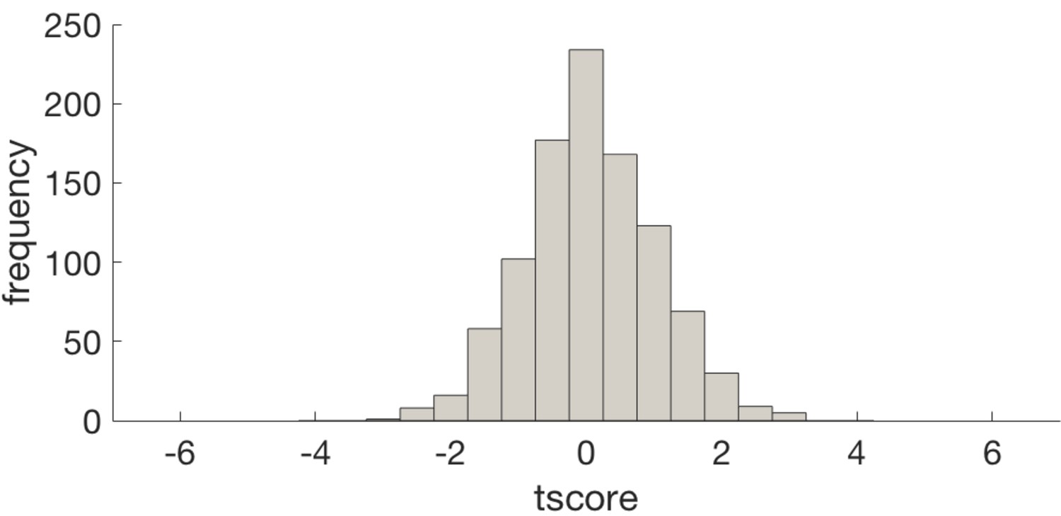
Histogram of t scores for the effect of entropy on representation strength (GLM4) for null data produced by shuffling voxel identities prior to PCA.
This demonstrates that the dimensionality reduction does not introduce bias in to the result. The histogram is centred about 0 and the t score of our analysis (−6.8) is off the distribution.
Figure 3 with 6 supplements
Neuromodulatory systems as a candidate mechanism for increasing flexibility of belief representations.
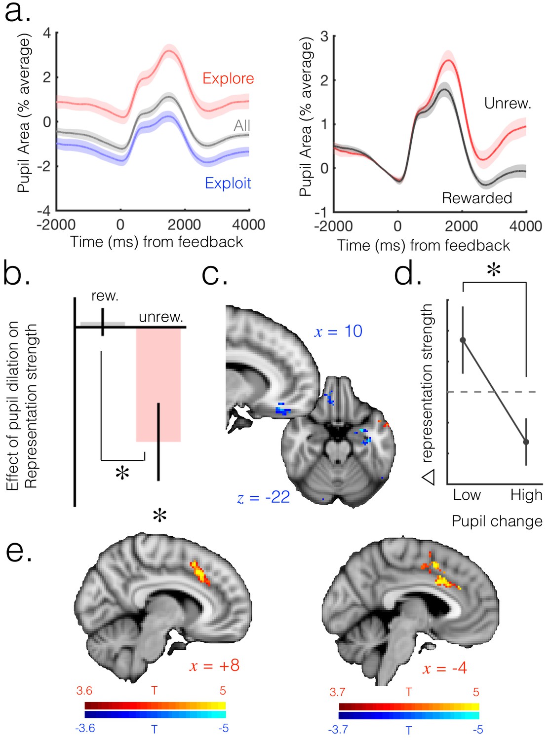
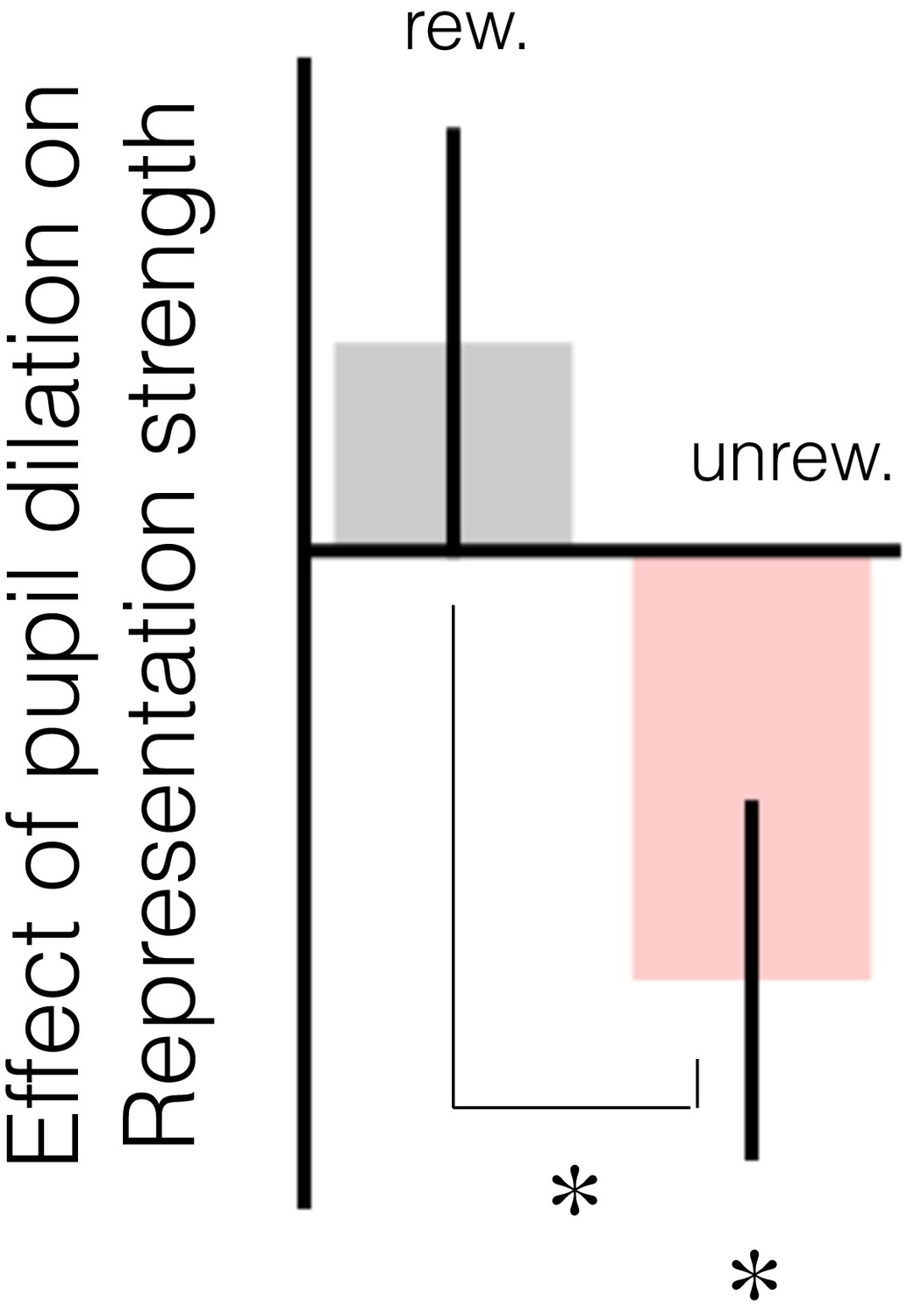
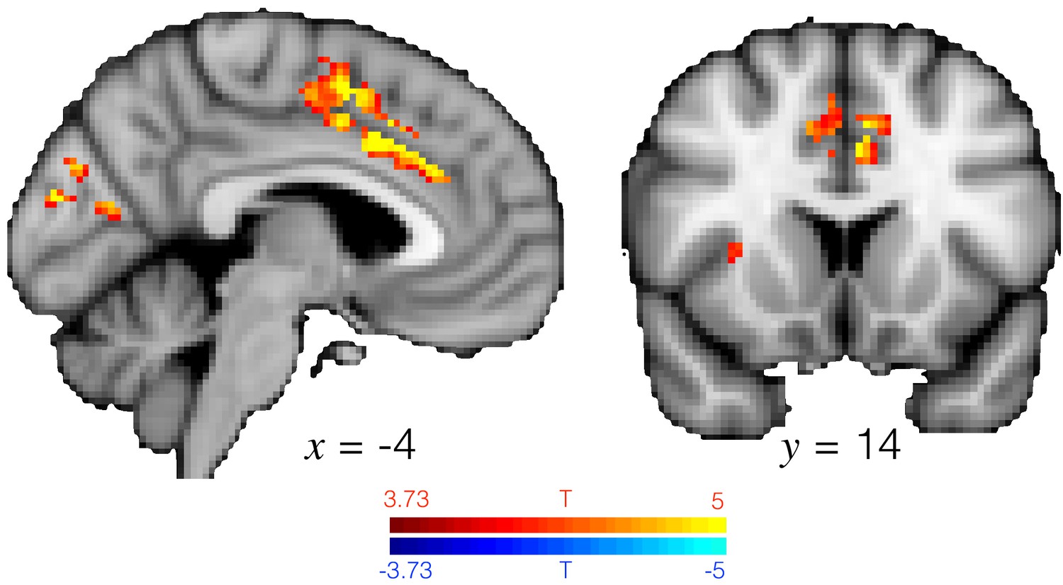
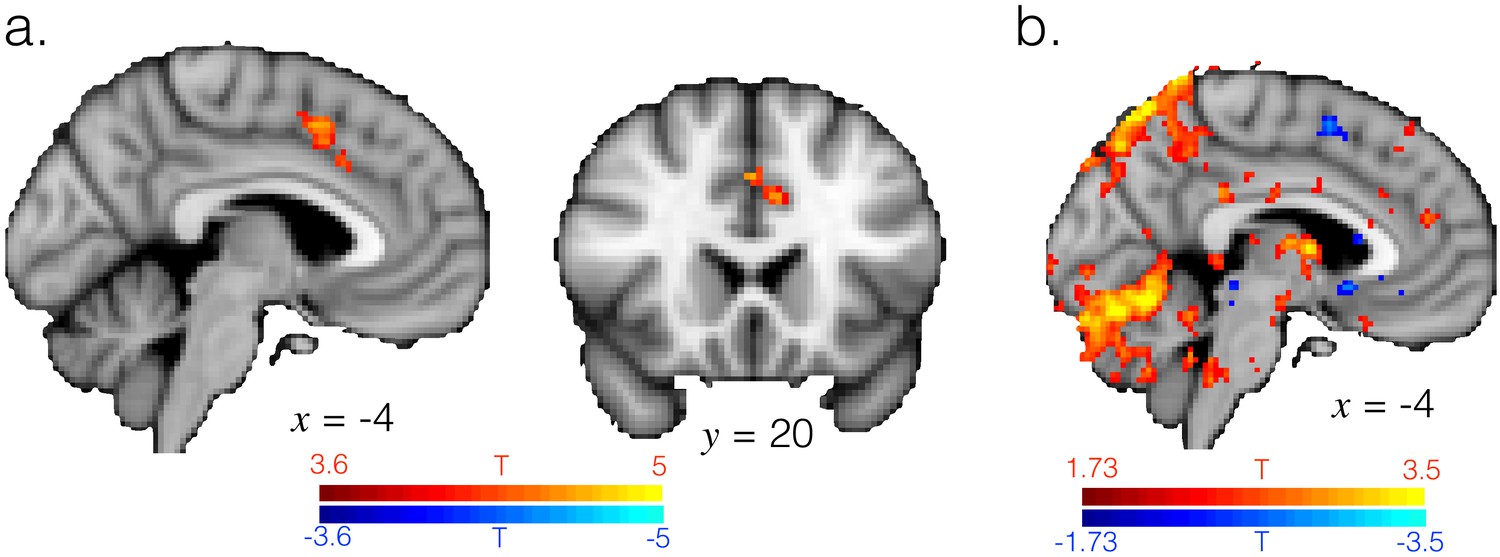
(a) Pupil size mean timecourses throughout a trial. Left: mean timecourses shown for all trials as well as trials split according to whether they were explore or exploit trials, revealing a larger pupil size in exploration than exploitation. Right: splitting trials according to whether the trial was rewarded or not reveals a sustained increase in pupil size following omission of reward. Shaded regions denote SEM. (b) Change in pupil diameter predicts changes in representation strength in mOFC on exploit trials. Beta weights for the effect of change in pupil diameter on change in representation strength are significantly below zero. This is true only on trials when reward was omitted. Error bars are SEM. (c) Performing this analysis as a whole brain reveals, again, a relatively localized effect in mOFC (t score map shown, thresholded at p<0.01, uncorrected; analysis performed on unrewarded exploit trials). (d) Median split on unrewarded exploit trials reveals that on trials when pupil change is high, change in representation strength is more negative than when pupil change is lower, in mOFC. Error bars are SEM. (e) Left: ACC region active when model entropy increased. Right: ACC region in which activity predicted changes in pupil dilation, over and above the effect of increase in model entropy and mean brain activity. Both thresholded at p<0.001 and corrected for multiple comparisons.
Figure 3—figure supplement 1
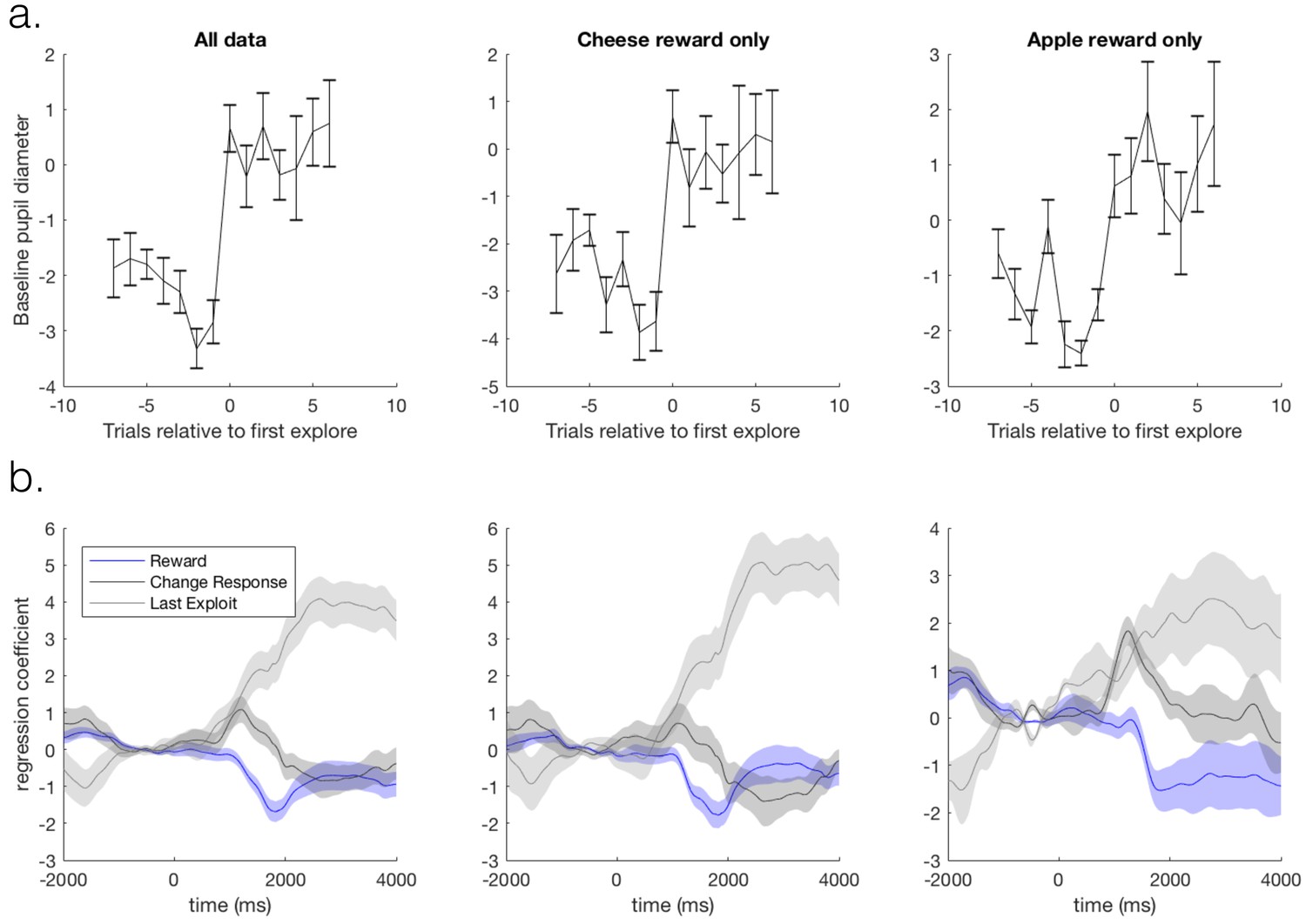
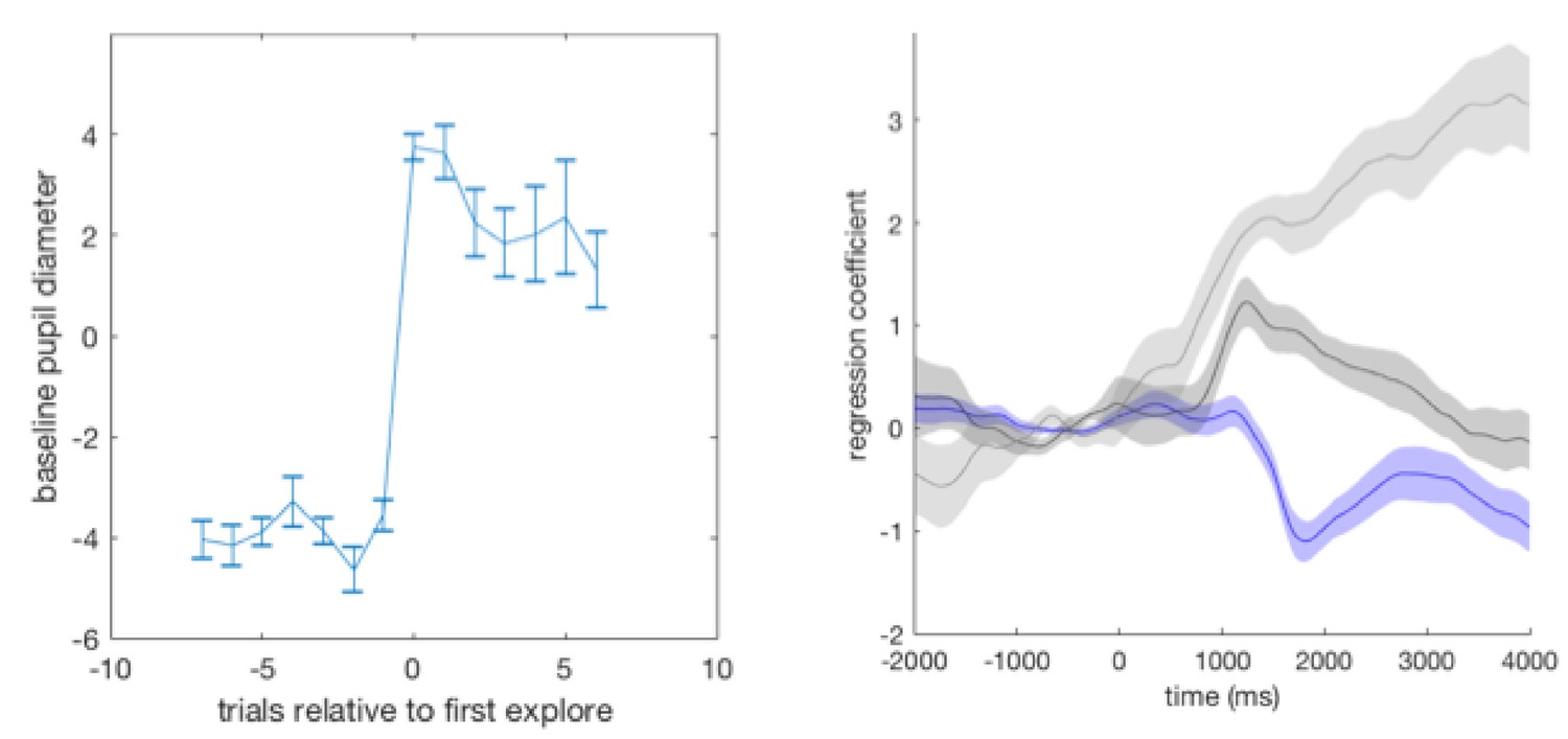
Task-related pupil size changes are not explained by outcome stimulus type.
We checked our results could not be explained by differences in luminosity between outcomes signalling reward vs. no reward. We counterbalanced the stimuli signalling rewarding vs. non-rewarding outcomes across participants: half the participants received a cheese stimulus as the rewarding outcome and apple stimulus as the unrewarding outcome, and the other half of participants received the converse. We analyse the pupil data from the behavioural session that each participant completed prior to the fMRI session, and split the participants according to the stimulus outcomes they received. We analyse the sixteen participants that entered pupil-brain analyses (ten received cheese as a reward, and six received apples as reward). We demonstrate that although noisier due to reduced power, pupil dilations to task factors are qualitatively the same when either the cheese or the apple was the rewarding outcome. We demonstrate this with two analyses. (a) First, by performing an analysis looking at the baseline pupil size on trials around transitions from exploitation to exploration. Mean baseline pupil size (again pupil size expressed as % of mean of that session) is presented as a function of trials around a transition from exploitation to exploration. A marked one trial increase in pupil size was observed as participants transitioned from exploitation to exploration (left panel), as has been previously observed (Jepma and Nieuwenhuis, 2011). Although noisier due to reduced power, this result was true when data was split according to either outcome identity type (cheese or apples; middle and right panels, respectively). Error bars are SEM. (b) Second, by constructing a GLM with regressors: reward, changing response on the next trial, switching in to exploration, as well as a main effect regressor, and performing a timeseries analysis with this GLM on all data and on data split according to stimulus outcome identities. Mean beta weights for the effect of the regressors in the GLM on pupil size are plotted as a function of time relative to outcome delivery. The data on each trial was normalised before performing the regression by demeaning the one second preceding outcome delivery. A constriction following reward delivery, a small dilation on trials on which participants changed their choice on the subsequent trial, and a large dilation when switching from exploitation in to exploration was observed. Again it can be observed that the results are qualitatively similar regardless of outcome identity type (middle and right panels). Shaded regions are SEM.
Figure 3—figure supplement 2
The relationship between change in baseline pupil diameter and change in representation strength in mOFC replicates in explore trials.
The figure has the same notation as Figure 3b in the main text. When performing this regression (GLM6) on explore trials, whether participants changed their response on the subsequent trial was added as a coregressor.
Figure 3—figure supplement 3
ACC activity explains changes in baseline pupil size across all trials.
T-statistic map showing where univariate brain activity explains changes in baseline pupil size, as in GLM8. Analysis performed in a grey matter mask, hence the streak in the activation. Similar to Figure 3e in the main text except across all trials. Image thresholded at p<0.001; corrected for multiple comparisons.
Figure 3—figure supplement 4
ACC is engaged when transitioning from exploitation to exploration.
(a) T-statistic maps for the regressor for switching from exploitation to exploration, as in GLM2 (note this is variance explained by the regressor over and above that explained by the other regressors in GLM2, such as changing response and reward). Image thresholding at p<0.001; corrected for multiple comparisons. (b) T-statistic map at a more liberal threshold of p<0.05, voxelwise and uncorrected, for the regressor for switching from exploration to exploitation, showing this transition does not engage ACC. Hence ACC transition-related activity appears to be specific for switching from exploitation to exploration and not vice versa.
Figure 3—figure supplement 5
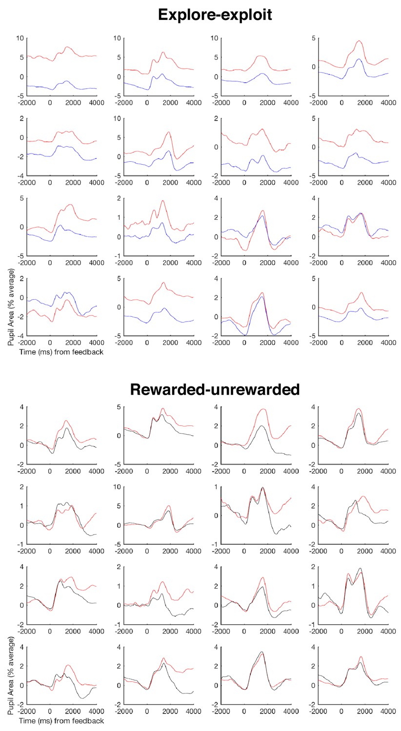
Individual pupil effects.
Here we show – as requested by a reviewer – individual pupil effects, since pupil effects are prone to strong individual differences. We present the mean timecourse for each participant for both of the two pupil effects presented in Figure 3a, namely splitting by exploit (red trace) and explore (blue trace) trials, and splitting by rewarded (red trace) and unrewarded (black trace) trials. Each panel denotes the effect for each of the 16 participants that entered the pupil analyses in Figure 3. Notations are the same as in Figure 3a.
Figure 3—figure supplement 6
Breaking central fixation does not alter pupil effects.
Figure notation the same as that in Figure 3—figure supplement 1, and analyses presented are the same, but having removed trials on which central fixation was broken. We instructed participants to maintain central fixation throughout the task. For technical reasons, the quality of the gaze location data from the fMRI session was too poor to use, so we were unable to determine whether fixation was broken. However, we did have good quality gaze location data from the behavioural session. Repeating the analyses presented in Figure 3—figure supplement 1 having removed trials containing eye movements reveals the results are qualitatively the same and quantitatively very similar to those results when trials on which central fixation was broken are not removed (as in Figure 3—figure supplement 1).
Appendix 1—figure 1
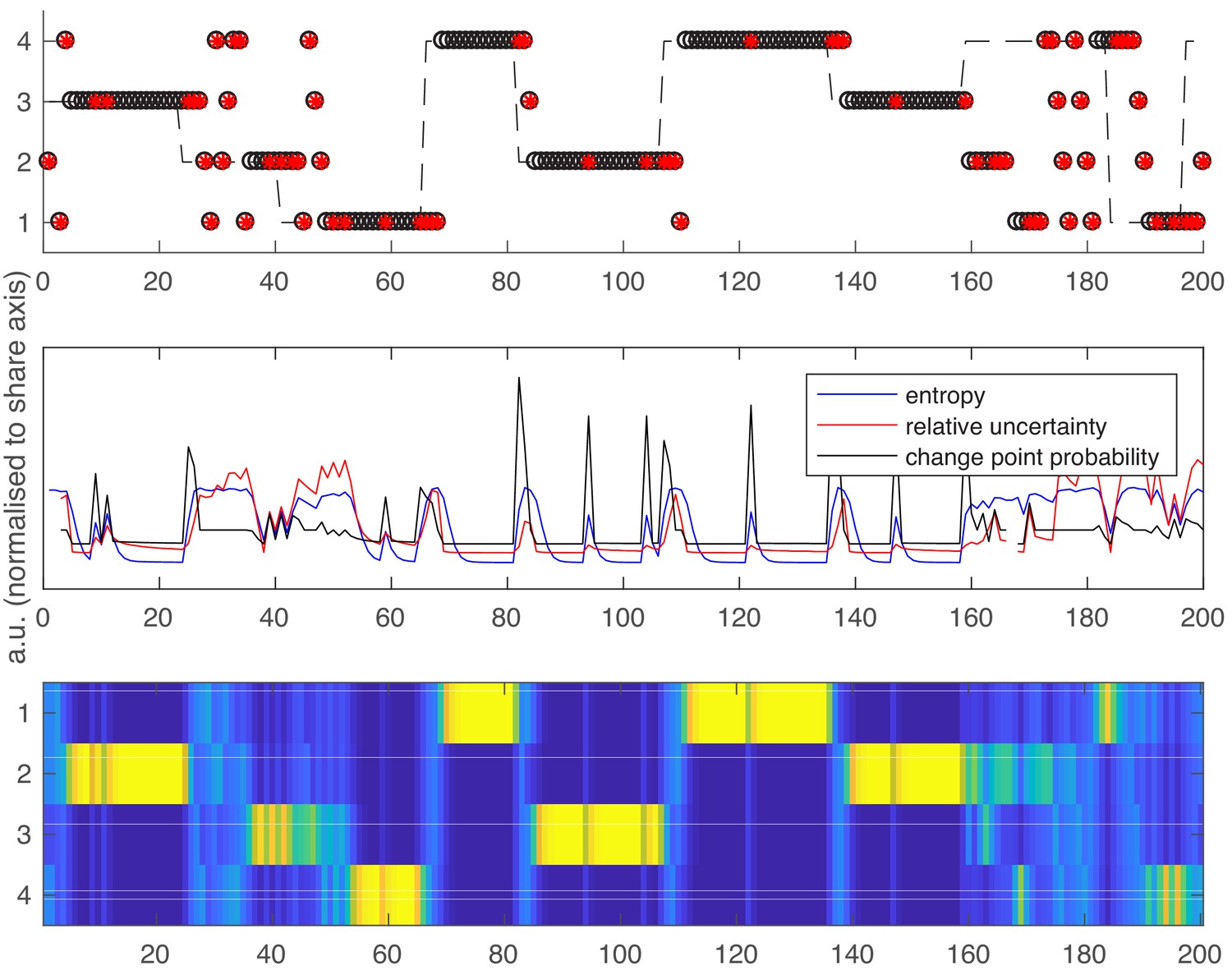
Following the same layout as Figure 1 in the main text.
Top panel – an example schedule for one participant/run. Y axis values 1–4 are the possible high reward locations, x axis values are trials. The dashed line shows the ground truth high reward location over time. Open black circles are participants’ choices; red dots are reward omissions. Middle panel - Entropy, relative uncertainty and change point probability measures, normalized for comparison. Note that CPP peaks rapidly after reward omission but also falls off rapidly, whilst entropy and relative uncertainty integrate multiple feedback events. Bottom panel – the probability distribution across candidate high reward locations (bright colors are higher probabilities).
Appendix 1—figure 2
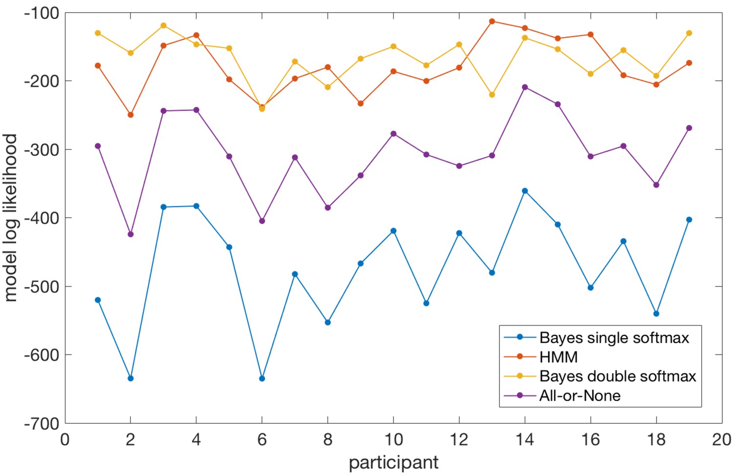
Model log likelihoods for each participant and each model, based on predicting participants’ choices across all trials.
Taken together, the model comparison suggests that the Bayesian model, when allowed to adopt different softmax policies in explore and exploit phases, performs very comparably to a model fitted directly to participants’ behaviour (the HMM). Importantly, because the Bayesian model simulates latent states of belief uncertainty (model entropy, relative uncertainty) even when behaviour is held constant during exploitation periods, it provides useful information over and above that given by the HMM (which does not model belief uncertainty at all). A second notable point is that the Bayesian model (with double softmax policy) does predict participants’ behaviour during explore periods. In contrast, the all-or-none model (which performed much worse than the Bayesian model with double softmax policy) sets an upper bound on the model log likelihood that could be achieved if behaviour in the explore period was random (as the probability of the chosen option during exploit periods is one and therefore model log likelihood is maximized in these periods).
Appendix 1—figure 3
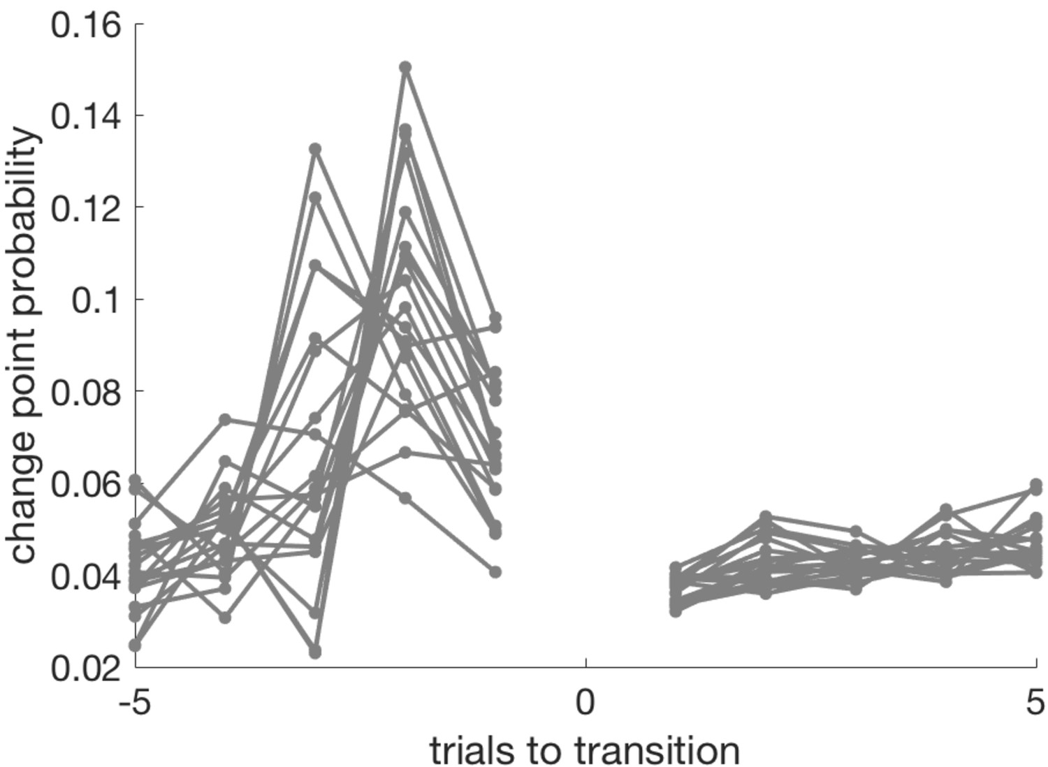
Change point probability in the trials leading up to, and following, the transition from exploit- to explore phase.
The last exploit trial is coded as −1, the first explore trial as +1 (there is no trial zero in this plot). CPP peaks on the penultimate trial of the exploit block, or the trial before that.
Appendix 1—figure 4
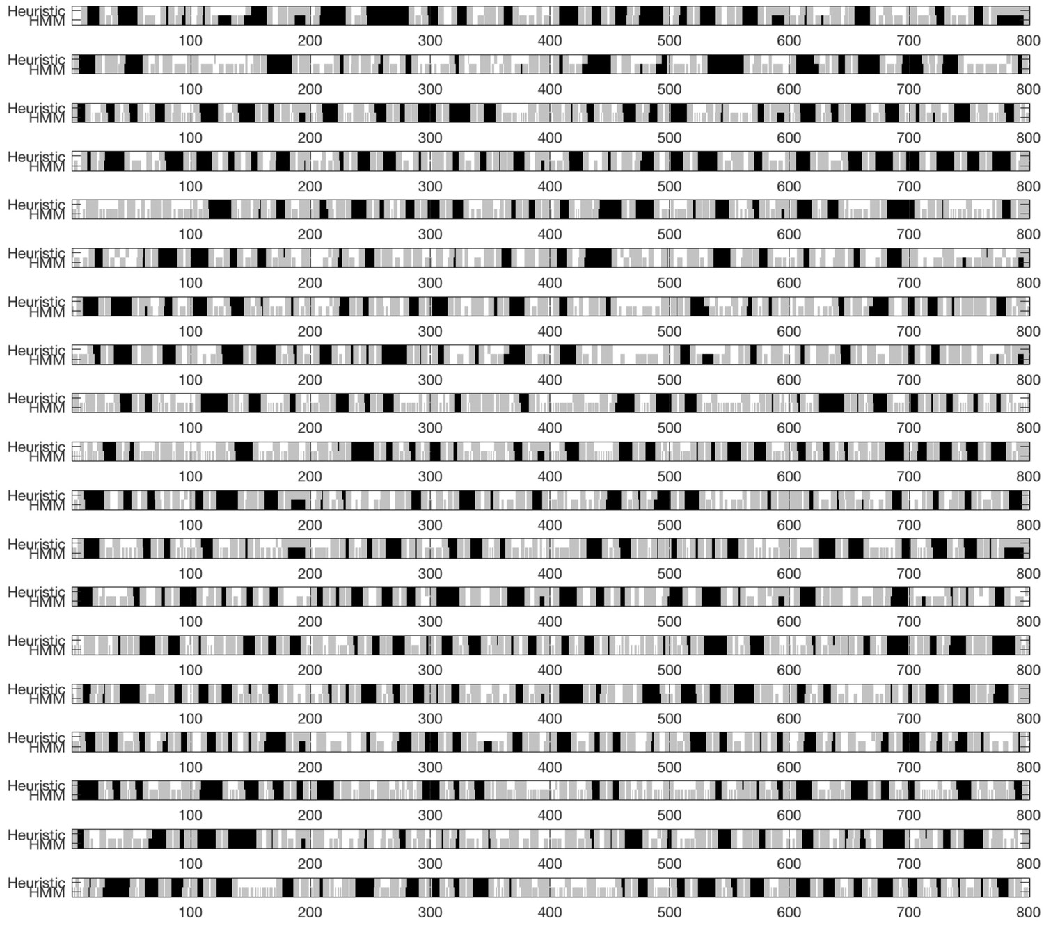
Explore and Exploit phases extracted by the Ebitz model.
Trials classified as ‘exploit’ (light grey) and ‘core exploit’ (dark grey) using our heuristic method (top) and the HMM method (bottom) for each of the 19 participants included in the main analysis. The HMM method tends to classify more trials as ‘exploit’ but because these are often short blocks, the trials classified as ‘core exploit’, used in all the multivariate analyses in the paper, are very similar for both classification methods.
Author response image 1
Additional files
-
Source code 1
MATLAB code for the Bayesian model in Figure 1, and the behavioural datasets to which the model was fit.
- https://doi.org/10.7554/eLife.39404.017
-
Transparent reporting form
- https://doi.org/10.7554/eLife.39404.018
Download links
A two-part list of links to download the article, or parts of the article, in various formats.
Downloads (link to download the article as PDF)
Open citations (links to open the citations from this article in various online reference manager services)
Cite this article (links to download the citations from this article in formats compatible with various reference manager tools)
Control of entropy in neural models of environmental state
eLife 8:e39404.
https://doi.org/10.7554/eLife.39404


