A high-throughput neurohistological pipeline for brain-wide mesoscale connectivity mapping of the common marmoset
- RIKEN Center for Brain Science, Japan
- Cold Spring Harbor Laboratory, United States
- Indian Institute of Technologies, India
- Johns Hopkins University, United States
- Monash University, Australia
- Australian Research Council Centre of Excellence for Integrative Brain Function, Australia
- Central Institute for Experimental Animals, Japan
- Keio University School of Medicine, Japan
Figures
Figure 1 with 1 supplement
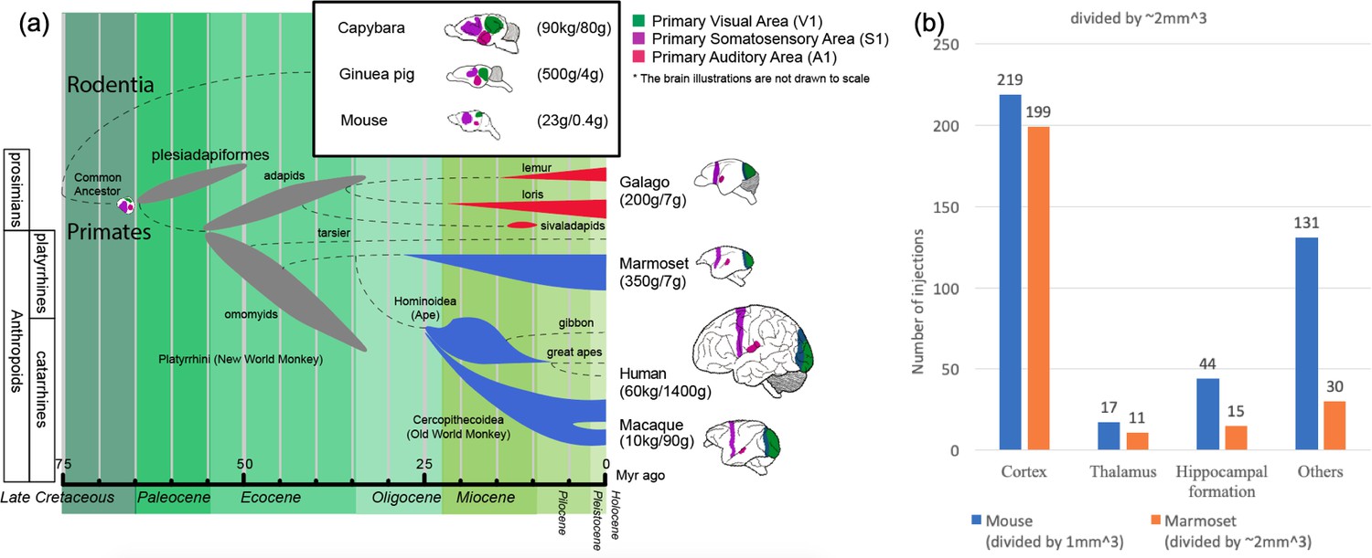
Phylogenetic tree of extinct and extant primates and numbers of injection sites achieved (in grid-based tracer mapping) for mouse and marmoset.
(a) Phylogenetic tree (Benton et al., 2009; dos Reis et al., 2014; dos Reis et al., 2012; Janecka et al., 2007; O'Leary et al., 2013; Mitchell and Leopold, 2015; Springer et al., 2011; Wilkinson et al., 2011) showing the ancestral history of extinct and extant primates, after divergence from the common ancestor with rodents (top right inset box) ca. 75 million years (Myr) ago. The bottom bar shows geological eras. Thickness of spindle shaped areas in the evolutionary tree indicate prosperity (estimated population and numbers of species) of the group along the history in extinct (gray) prosimian (red) and simian (blue) primates. Each bifurcation represents the species divergence, although the divergence time typically has a wide range and remains controversial. Primates diverged into platyrrhini, the New World Monkey, and catarrini, around 38.9–56.5 million years ago. Catarrini further evolved into Ape, including humans, and Old World Monkey as well as macaque monkeys 25.1–37.7 million years ago. Sketches of the brain in each species are shown on the right, next to their species name. The colored areas in the various brain illustrations indicate the primary visual area as green, somatosensory as purple, and auditory areas as red; each represents an extant primate (bottom right row) and rodent (top inset box) species’ body weight (first numbers in brackets) and brain weight (last numbers in brackets) sizes (Buckner and Krienen, 2013; Krubitzer and Dooley, 2013; Krubitzer and Seelke, 2012). Phylogenetic tree adapted from Masanaru Takai (Takai, 2002). (b) Fractional brain region volumes, and numbers of injection sites used in grid- based injection plans for marmoset (Woodward et al., 2018) and mouse (Allen institute for brain science, 2017). Bar plots show the number of grid-injection sites within the displayed compartment in each species, assuming a spacing between injection sites of ~1 mm isometric in mice, and ~2–3 mm isometric in marmosets.
Figure 1—figure supplement 1
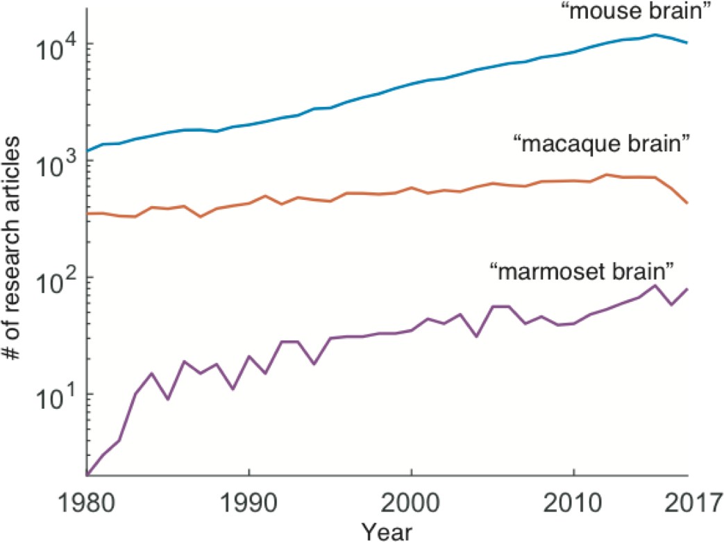
Number of research articles comparing mouse, macaque and marmoset in 1980-2017.
Marmoset brain research articles increase 1980–2017 compared with mouse and macaque brain research listed on PubMed (www.ncbi.nlm.nih.gov/pubmed). Number of articles are plotted in logarithmic scale for results returned from searching the keywords of ‘mouse brain’, ‘macaque brain’, or ‘marmoset brain’.
Figure 2 with 1 supplement
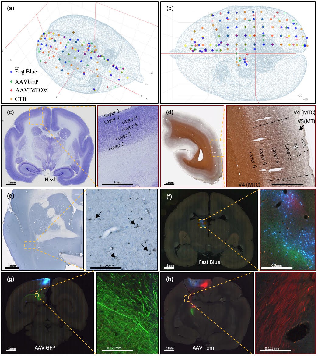
Current injection sites covered, example of staining methods, and different colors of marker in coronal brain sections.
(a, b) Current successful injection sites using 2×2×2 mm grid spacing in the marmoset cortex in (a) 3D and (b) 2D dorsal view, in stereotaxic coordinates (Paxinos et al., 2012). (b) Current successful injection sites. Each tracer is represented with a different color of marker: blue: Fast Blue; green: AAV-GFP; red: AAV-tdTOM; brown: CTB. Two tracers, one anterograde and one retrograde, are injected at each site. (c–h) Sample coronal brain section images of four series. (c) A coronal section after Nissl staining is shown with increasing magnification. Around Area 3a (magnification box), six cortical layers and the white matter are clearly differentiable based on cell body density. (d) A coronal section of the left hemisphere after silver staining showing myelin. Around Visual area V4T (Middle Temporal) crescent; magnification box), layers I-VI can be clearly characterized based on the myelin fiber density. Heavy myelination can be seen in layer three and continues into layer 4–6 with clear inner and outer bands of Baillarger. (e) Partial coronal section after immunohistochemistry treatment for CTB. After injection into Area 10, CTB labeled neurons were found in the claustrum (magnification box). The arrows indicate CTB- labeled cells at 0.125 mm. (f–h) Coronal sections in different parts of the brain showing fluorescent tracers including (f) retrograde tracer Fast Blue (g) anterograde tracer AAV-GFP, and (h) anterograde tracer AAV-tdTOM.
Figure 2—figure supplement 1
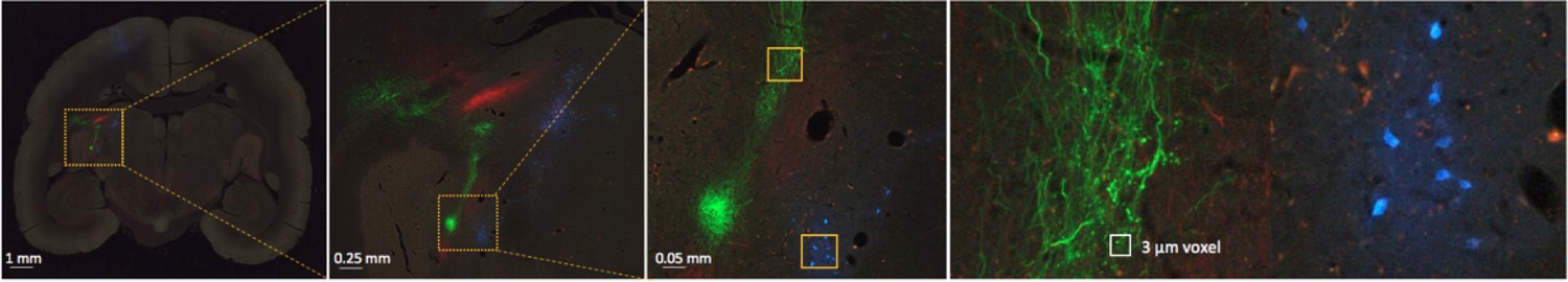
Example of a coronal section of the brain showing fluorescent tracers in high magnification.
We have obtained each coronal section in 0.46 µm per pixel with 20 µm section thickness. The mesoscale level image (high magnification on the right) shows clear projections in the thalamus with labeled cells/axons in representative subcortical regions.
Figure 3
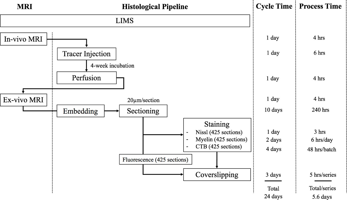
The workflow of the experimental pipeline and the processing time for one marmoset brain.
Arrows show the sequence of individual experiments. A custom-made LIMS (Laboratory Information Management System) performs housekeeping for the entire process and constitutes an electronic laboratory notebook. The entire brain is sectioned into ~1700 sections,~400 in each series. Each series include ~295 slides, comprising of 1/3 of the slides with two brain sections mounted and 2/3 with one brain section/slide. Coverslipping includes the drying and clearing stages. The processing time does not include the overnight waiting period after sectioning in each batch. The overnight incubation time is excluded in the CTB procedure as well as the overnight dehydration in a myelin stain. Process Time on the right shows the time involved in processing each experimental step, in hours. The Cycle Time (in days) shows the total time required to initiate and finish the entire procedure from start to finish, including quiescent periods, before commencing the procedure for another brain. Total time on the bottom is not a summation of the individual procedure times above because of parallel, pipelined processing which reduces total processing times. For example, when Nissl series are being processed in the automatic tissue staining machine for Nissls, CTB and myelin staining can be performed simultaneously at other workstations.
Figure 4
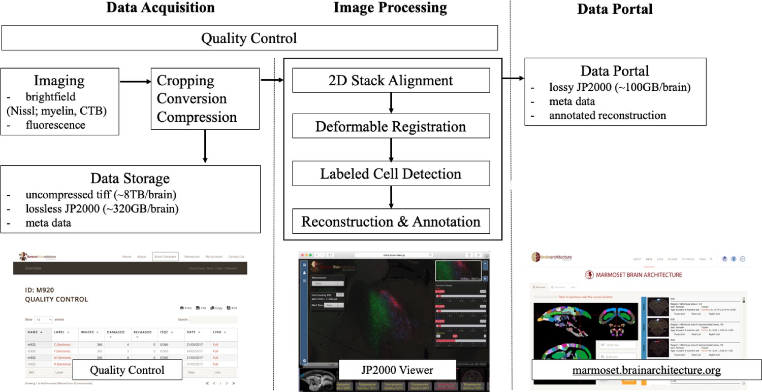
A flow chart showing the workflow of the computational pipeline, from data acquisition to image processing and finally dissemination on the public data portal.
Arrows show the data flow. A quality control system is implemented at every stage of the pipeline until final data release. The display of the data portals is to allow interactive service. (a) A quality control site (snapshot on the bottom left) which helps improve the pipelines process speed and manually flags unnecessary sections to avoid further post-processing. (b) An Openlayer 3.0 JPEG2000 viewer (snapshot on the bottom middle) including several controls such as dynamic range, gamma, measurement and auto cell detection tool to allow for a users’ interpretation (Lin et al., 2013). (c) The data portal site (snapshots on the bottom right) helps to host all successful and processed dataset for publishing purposes.
Figure 5

3D deformable registration and atlas mapping of all four series.
The Brain/MINDs atlas was registered with ex-vivo MRI volume, and subsequently registered to target Nissl series (a) The shaded areas indicate missing sections at the end of processing (quality control). Other series including (b) myelin, (c) CTB and (d) fluorescence series were cross-registered to target Nissl series, and aligned with the atlas annotations. Only gray scale images are shown and they are sufficient for the registration process. Sample sections in transverse (left), sagittal (middle), and coronal (right) were shown for each series.
Figure 6
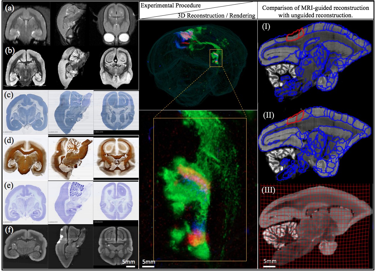
Different stages of image acquisition, 3D reconstruction, and MRI-guided registration in this experimental protocol.
(left) Views of one marmoset brain after each experimental protocol. (a) in-vivo MRI (b) ex-vivo MRI (c) CTB staining (d) myelin staining (e) Nissl staining (f) fluorescence imaging. Coronal, sagittal and transverse planes at the same (MRI) or consecutive sections (staining series) are shown with 3D registration and reconstruction. (middle) A 3D visualization of the fluorescent tracer projection. Simultaneous anterograde (red, green) and retrograde (blue) tracing reveals a reciprocal connection between the dorsal medial visual area (injection site) and the thalamus (anterograde projection and retrograde cell labeled sites) especially lateral posterior nucleus and lateral pulvinar. The connectivity can be observed with this 3D visualization which shows the pathway of tracers in through the brain volume. (right) Comparison of MRI-guided reconstruction with unguided reconstruction. I: the target Nissl stack reconstruction by unguided piecewise neighbor-to-neighbor alignment. II: the MRI-guided reconstruction. III: same- subject T2-weighted MRI.
Figure 7

A part of the connectivity matrix identified with tracer injections in one sample brain.
The retrograde tracer Fast Blue was injected in V6 and found in high density in several regions such as lPul and A31. AAV-GFP was injected in V1 and AAV-TdTOM in V6 and show clear projections to the thalamus and other visual areas. Each row contains all projections to different brain regions originating from those AAV tracers. The magnified images highlight some clear origin/projections from the injected tracers in the connectivity matrix.
Appendix 3—figure 1
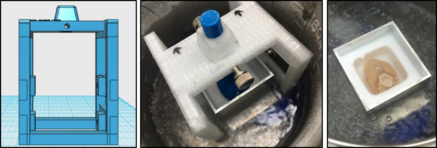
Rectangular base mold was designed and printed to serve as a freezing platform.
The freezing platform was used to control the position of the brain mold to the base mold during freezing. The positioning bar is adjustable to allow ease of insertion and removal of the brain mold from the base mold.
Appendix 4—figure 1

Modified cryostat chamber to accommodate for larger brain block.
(a,b) Additional stage shown in pink was attached to the original cryostat stage to increase the room space and to aid in stabilization of the cryostats chuck and blade. (c) a four row UV-LED device to provide UV intensity across the surface of the slides by an on-off timer controller using a Raspberry Pi.
Appendix 6—figure 1
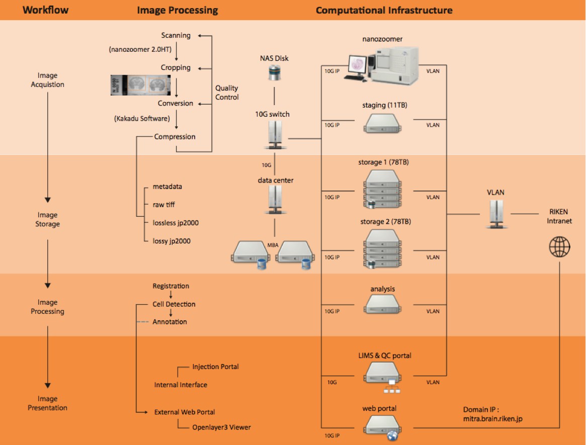
Computational pipeline with the network structure to perform a high-throughput data flow and process.
There were four steps of workflow involved in this pipeline including image acquisition, storage, processing and presentation. With these steps, generating a whole marmoset brain dataset with high production rate and superior system performance for large data communication was possible. Each server node was connected to one 10G network for data communication and one external network for remote access.
Appendix 7—figure 1
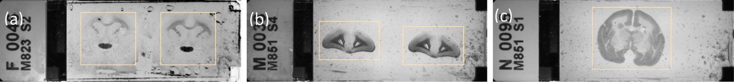
Example of a Nanozoomer macro image determining the cropping ROIs.
(a) fluorescence slide (b and c) brightfield slides shown with yellow cropping box.
Appendix 8—figure 1

A pipeline processing rate with four series staining (fluorescence, Nissl, myelin, CTB) based on the latest 10 datasets.
Each series starts with 100% full rate (based on the calculation from ex-vivo MRI and the number of sections needed as well as calculated by measuring at 20 μm each) and reduces by a percentage based on unavoidable reasons such as poor staining or section peeling. The figure shows that there is high processing rate starting with Nissl (91%), fluorescence (89%), CTB (84%), to myelin (81%). The average processing rate is 87% in total.
Appendix 9—figure 1
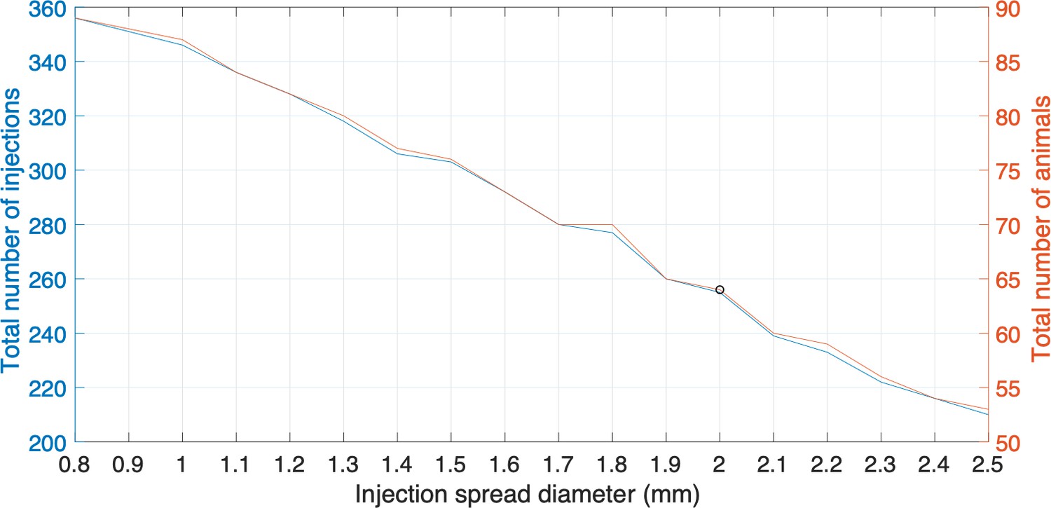
Plots representing the total number of injections, the number of animals needed and injection spread diameter (mm).
Each plot represents the different sizes of injection spread in diameter (mm); the right side y-axis represents the total number of animals required to be involved in the experiments; the left side y-axis represents the total number of injections. The black circle is the cutoff where a 2 mm diameter injection spread requires 255 tracer injections throughout a total of 64 marmoset brains. The cutoff represents a reasonable balance between minimal animal use versus maximum number of tracers that can be used in this experiment.
Appendix 10—figure 1
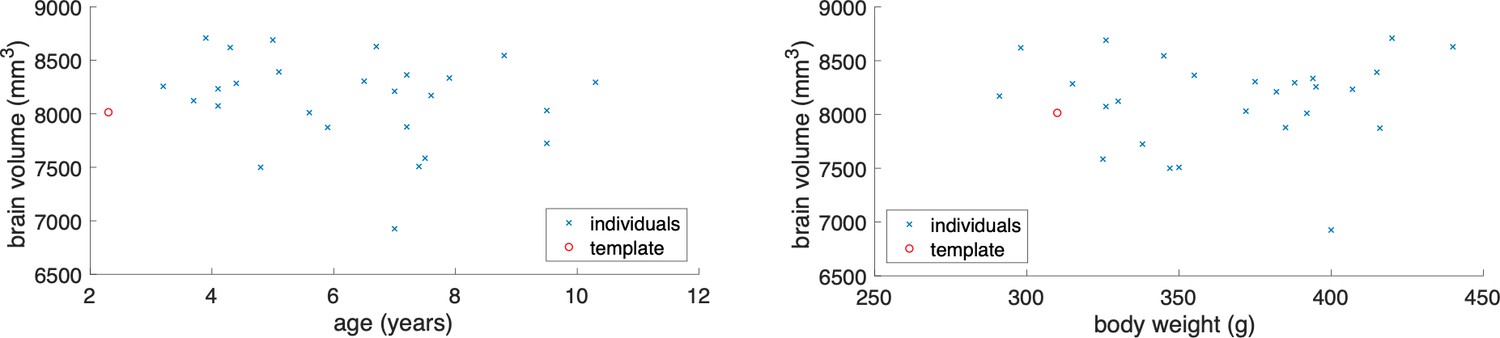
Relationship between whole brain volume and age or body weight.
The left plot shows individual marmoset variation between whole brain volume and age in comparison to the Brain/MINDS template. The right plot shows individual marmoset variation in comparison to body weight and to the Brain/MINDs template. The red circle represents the Brain/MINDs template brain and the blue crosses represents individual animals in this experiment. These plots show no significant relationship between the template brain and individual experimented brains.
Appendix 10—figure 2
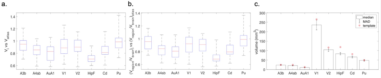
Comparison of individual variability of representative brain regions against the template brain.
(a) Box plots of ratio of each brain region’s volume in individual animals against its volume in the template brain, where the red line shows the median, the lower and upper bound of the box shows the 25th and 75th percentile data, respectively, and the whiskers extend to most extreme data points. A ratio of 1 means the same volume between the brain region in the animal(s) involved in the current project and the template brain. A ratio lower/higher than one means smaller/larger brain region in the animal in the current project compared with the template brain. (b) Box plots of each brain region’s proportion in the entire brain in individual animals against the proportion in the template brain. Similar to (a), the red line shows the median, the upper and lower bound of box shows the 75th and 25th percentile data, and the whiskers show the most extreme data. A ratio of 1 means the same proportion of the brain in the individual compared with the template brain. (c) Bar plot of the absolute volume of individual brain regions across different animals. Height of the bar shows the median and the error bars show the MAD.
Appendix 10—figure 3
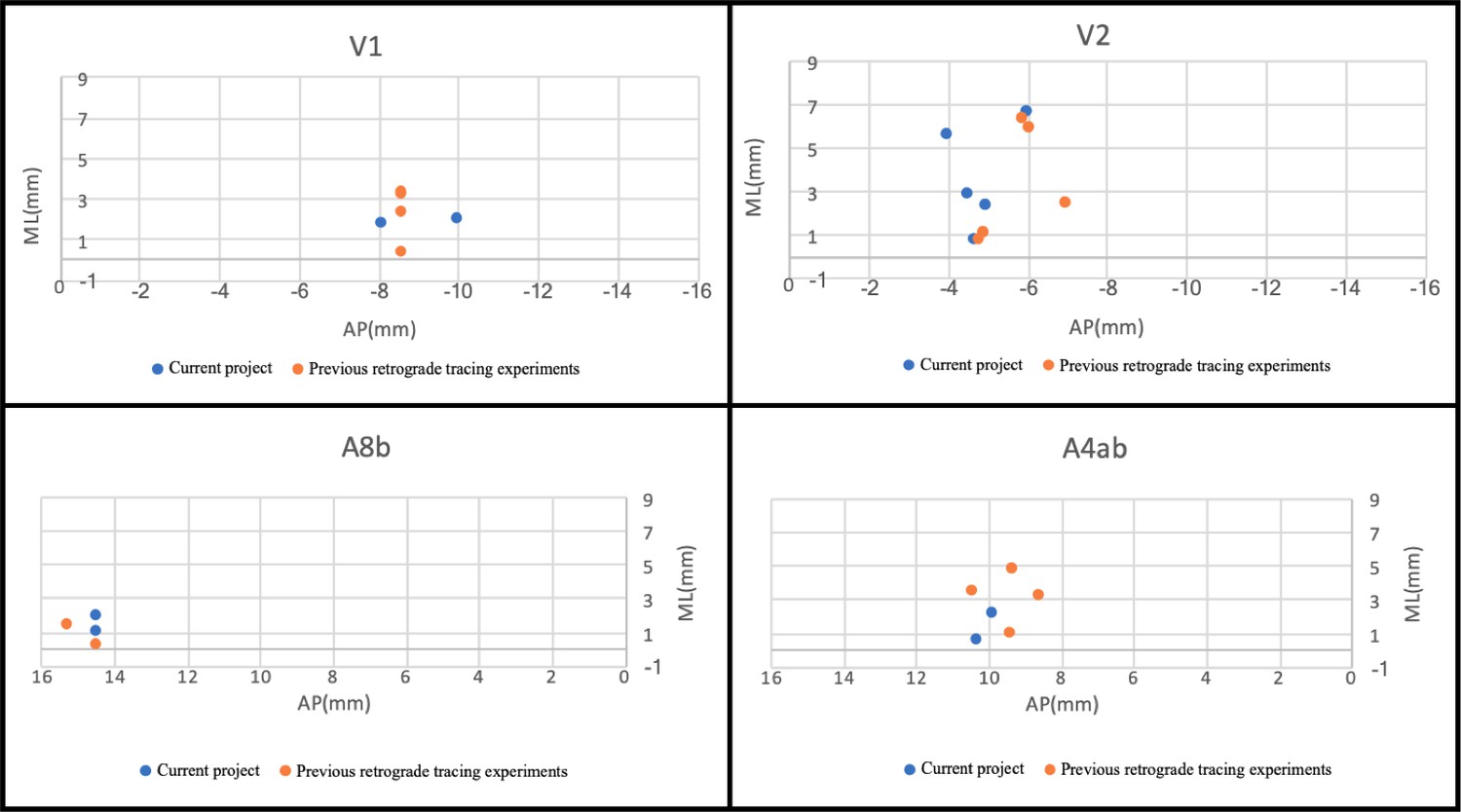
Transverse projection of the injection locations between individual brains in the current project and previous retrograde tracing experiments.
The similar plots (injections) presented here in V1, V2, A8b, and A4ab suggests that the current grid method is feasible and can be further analyzed across other collaborative projects.
Videos
Video 1
The registration process permitted brain surface reconstruction.
A brain fully reconstructed using MRI guided registration with process and cell detection. A clear pathway is seen from the tracer traveling from region to region in this 3d visualization of projections. Virtual cuts in planes of sections other than the original coronal sections are also shown.
Tables
Table 1
Past and present summary of historical tract-tracing studies in macaque and marmoset monkeys.
Three resources of macaque monkey brain connectivity are shown. Felleman and Van Essen (Felleman and Van Essen, 1991) and CoCoMac each surveyed a set of studies to generate the connectivity matrix (full reference list in Supplementary file 2). Note that CoCoMac is inclusive of the work collected in Felleman and Van Essen (Felleman and Van Essen, 1991). Around 235 injections lack tracer direction information. Markov et al. (2014) was a single study using only the retrograde tracer to generate the connectivity matrix as well as quantifying the connection strengths. We have surveyed 35 marmoset brain tracing studies that contain 428 tracer injections including both anterograde and retrograde tracers. A complete connectivity matrix is not yet available for the marmoset brain. To date, the most comprehensive marmoset brain connectivity resource available online (http://monash.marmoset.brainarchitecture.org) includes 143 retrograde tracing studies. As part of the current pipeline, we have placed over 188 tracer injections including both anterograde and retrograde tracers. For both macaque and marmoset brain injections, bidirectional tracer injections were double counted as one anterograde and one retrograde tracer injection.
| Data | Species | Injections | Anterograde tracer | Retrograde tracer | Connectivity matrix | Source | |
|---|---|---|---|---|---|---|---|
| Journal papers | No whole-brain image data | Macaque | 370 | 153 | 217 | 33 × 33 | Felleman and Van Essen, 1991 (52 studies) |
| 3279 | 1429 | 1873 | 58 × 58 | CoCoMac (459 studies) | |||
| 39 | 0 | 39 | 29 × 91 | Markov et al., 2014 | |||
| Marmoset | 428 | 93 | 395 | - | 35 studies (Bibliography in supplement) | ||
| Whole-brain image data | Nissl images overlaid with cell locations (Rosa Lab data set) | Marmoset | 143 | 0 | 143 | - | Online |
| This paper: Whole-brain set of cross-modal serial sections (Nissl,Myelin, IHC, Fluoro)+MRI | 188 | 94 | 94 | - | This paper |
Appendix 10—table 1
Median and MAD of each metrics evaluating the brain region volume’s variability across animals.
The table shows some of the large components in the marmoset brain.
| Whole brain | 'A3b' | 'A4ab' | 'Aua1' | 'V1' | 'V2' | 'Hipf' | 'Cd' | 'Pu' | ||
|---|---|---|---|---|---|---|---|---|---|---|
| Vi | Median | 8234 | 23.76 | 21.40 | 10.91 | 235.76 | 105.04 | 83.64 | 66.26 | 48.55 |
| MAD | 351 | 2.38 | 2.46 | 1.41 | 36.70 | 12.71 | 7.42 | 7.75 | 5.93 | |
| Vi/Vatlas | median | 1.03 | 0.95 | 0.86 | 0.83 | 0.89 | 0.90 | 0.71 | 0.81 | 0.99 |
| MAD | 0.04 | 0.09 | 0.10 | 0.11 | 0.14 | 0.11 | 0.06 | 0.10 | 0.12 | |
| (V/Vbrain)i/(V/Vbrain)atlas | median | 1 | 0.96 | 0.85 | 0.81 | 0.92 | 0.91 | 0.68 | 0.80 | 0.99 |
| MAD | 0 | 0.10 | 0.09 | 0.10 | 0.12 | 0.10 | 0.07 | 0.09 | 0.11 |
Additional files
-
Supplementary file 1
List of target structures and number of injections.
- https://doi.org/10.7554/eLife.40042.013
-
Supplementary file 2
Reference list of trace tracing studies.
- https://doi.org/10.7554/eLife.40042.014
-
Transparent reporting form
- https://doi.org/10.7554/eLife.40042.015
Download links
A two-part list of links to download the article, or parts of the article, in various formats.
Downloads (link to download the article as PDF)
Open citations (links to open the citations from this article in various online reference manager services)
Cite this article (links to download the citations from this article in formats compatible with various reference manager tools)
A high-throughput neurohistological pipeline for brain-wide mesoscale connectivity mapping of the common marmoset
eLife 8:e40042.
https://doi.org/10.7554/eLife.40042


