Global warming reduces leaf-out and flowering synchrony among individuals

  1. Constantin M Zohner  Is a corresponding author
  2. Lidong Mo
  3. Susanne S Renner
  1. ETH Zurich (Swiss Federal Institute of Technology), Switzerland
  2. University of Munich (LMU), Germany

Abstract

The temporal overlap of phenological stages, phenological synchrony, crucially influences ecosystem functioning. For flowering, among-individual synchrony influences gene flow. For leaf-out, it affects interactions with herbivores and competing plants. If individuals differ in their reaction to the ongoing change in global climate, this should affect population-level synchrony. Here, we use climate-manipulation experiments, Pan-European long-term (>15 years) observations, and common garden monitoring data on up to 72 woody and herbaceous species to study the effects of increasing temperatures on the extent of leaf-out and flowering synchrony within populations. Warmer temperatures reduce in situ leaf-out and flowering synchrony by up to 55%, and experiments on European beech provide a mechanism for how individual differences in day-length and/or chilling sensitivity may explain this finding. The rapid loss of reproductive and vegetative synchrony in European plants predicts changes in their gene flow and trophic interactions, but community-wide consequences remain largely unknown.

Editorial note: This article has been through an editorial process in which the authors decide how to respond to the issues raised during peer review. The Reviewing Editor's assessment is that all the issues have been addressed (see decision letter).

https://doi.org/10.7554/eLife.40214.001

Introduction

The structure and functioning of ecosystems crucially depends on the timing of annually repeated life stages, such as leaf-out and flowering (Ims, 1990; Fitter and Fitter, 2002; Sherry et al., 2007; Thackeray et al., 2016). Anthropogenic climate warming is causing advanced leaf-out and flowering in both herbs and trees, and this is affecting growth and reproductive success (Menzel and Fabian, 1999; Chuine and Beaubien, 2001; Elzinga et al., 2007; Chuine, 2010). Warmer springs and summers are also causing leaf-out and flowering to spread out over longer periods because the sensitivity to changing abiotic conditions differs among species (Fitter and Fitter, 2002; Sherry et al., 2007; Zohner et al., 2017; Laube et al., 2014; Zohner et al., 2016). Leaf-out and flowering times might also spread out within species (CaraDonna et al., 2014), potentially reducing phenological synchrony among individuals. For leaf-out, inter-individual synchrony affects interactions with foliovores and competing plants (Hart et al., 2016). For flowering, reduced inter-individual synchrony should adversely affect gene flow by reducing cross-pollination and fruit set (Augspurger, 1981) and alter co-flowering patterns within communities (CaraDonna et al., 2014; Forrest et al., 2010). To detect such possible effects of climate warming on within-population synchrony, a range of herbs and trees, representing different leaf-out and flowering strategies, needs to be studied.

Here, we use a combination of climate-manipulation experiments, common-garden monitoring, and long-term Central European in situ observations to analyze effects of warming on intraspecific phenological synchrony. The long-term data were obtained from the Pan European Phenology Project (http://www.pep725.eu, hereafter PEP) and consisted of 12,536 individual time series (each minimally 15 years long), comprising the leaf-out times of nine dominant tree species and the flowering times of six tree species, four shrubs, and five herbs (see Materials and methods and the distribution of the sites in Figure 1a, Figure 1—figure supplements 1 and 2).

Figure 1 with 5 supplements see all
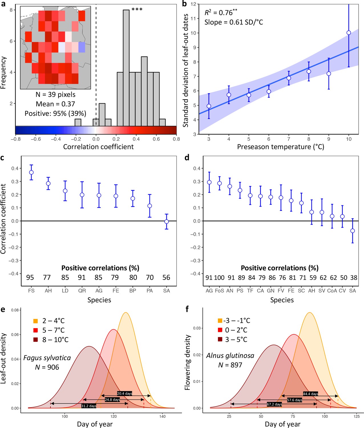
Loss of inter-individual synchrony in leaf-out and flowering with increasing temperatures.

(a) Frequency distribution showing the correlations between the standard deviation of inter-individual leaf-out times and spring temperature for Fagus sylvatica at 39 pixels (1° x 1° areas). Mean = Mean correlation coefficients across all sites (N) Positive = percentage of positive correlations and the percentage of statistically significant positive correlations (in parentheses). Inset shows a heat map of the correlations at the 39 pixels. (b) Effect of preseason temperature on the standard deviation of inter-individual leaf-out times (mean ± SEM) in F. sylvatica averaged across all years and sites. (c) (d) Mean Pearson correlation coefficients (± 95% confidence intervals) for the effect of spring temperature on the standard deviation of inter- individual leaf-out (c) or flowering times (d). Positive correlations = percentage of the total number of positive correlations. See Figure 1—figure supplements 1b and 2b for number of sites (1° x 1° areas) in which the relationship was analyzed. (e) (f) Distributions of inter-individual (e) leaf-out dates in F. sylvatica and (f) flowering dates in Alnus glutinosa under different spring temperatures. N = Number of available year x pixel (1° x 1° areas) combinations. To model the distributions (means and standard deviations), mixed-effects models were applied including site (pixel) as a random effect. See for distributions of all 20 analyzed species. AG, Alnus glutinosa; AH, Aesculus hippocastanum; AN, Anemone nemorosa; BP, Betula pendula; CA, Corylus avellana; CoA; Colchicum autumnale; CV, Calluna vulgaris; FE, Fraxinus excelsior; FoS, Forsythia suspensa; FS, Fagus sylvatica; FV, Fragaria vesca; GN, Galanthus nivalis; LD, Larix decidua; PA, Picea abies; PS, Prunus spinosa; QR, Quercus robur; SA, Sorbus aucuparia; SC, Salix caprea; SV, Syringa vulgaris; TF, Tussilago farfara.

https://doi.org/10.7554/eLife.40214.002

Results and discussion

To analyze the PEP data, the study area was divided into pixels of one-degree resolution (~110×85 km), and leaf-out synchrony (LOS) and flowering synchrony (FLS) in a given year were then calculated as the standard deviation of leaf-out or flowering date for all individuals within a pixel (note that the data were cleaned to ensure that observed individuals were the same between years; see Materials and methods). For each pixel and each phenological stage (leaf-out or flowering), we determined preseason as the period 60 days before the average leaf unfolding or flowering date within the respective pixel.

As expected, within pixels, species’ mean leaf-out dates were negatively correlated with preseason temperature (98% of observation series statistically significant at p<0.05), with a mean linear correlation coefficient of −0.76 ± 0.03 (mean ± 95% confidence interval), predicting an average advance of 4.3 ± 0.2 days per each degree warming. Similarly, in more than 99% of pixels, the mean flowering dates were negatively correlated with the preseason temperature (91% statistically significant at p<0.05), with a mean linear correlation coefficient of −0.75 ± 0.10, predicting an average advance of 4.6 ± 0.2 days per each degree warming.

Higher preseason temperatures had a negative effect on LOS in eight of the nine species (Figure 1c, Figure 1—figure supplement 1) and on FLS in 10 out of 15 species (Figure 1d, Figure 1—figure supplement 2). None of the species exhibited a positive effect. Across all species, preseason temperature negatively affected LOS in 78% of analyzed pixels (15% statistically significant at p<0.05), that is, the standard deviation of inter-individual leaf-out times increased by 0.45 ± 0.07 (mean ± CI) days per degree of warming, with a mean linear correlation coefficient of 0.19 ± 0.03. Significant positive effects of preseason temperature on LOS appeared in fewer than 1% of pixels. The species showing the strongest decline in LOS related to warmer preseason temperatures was European beech (Fagus sylvatica; Figure 1a): preseason temperature negatively affected LOS in 95% of analyzed pixels (39% statistically significant), with the standard deviation of inter-individual leaf-out times increasing by 0.61 ± 0.05 days per degree of warming (Figure 1b). When modelling the distribution of leaf-out dates within pixels, we found that preseason warming increases the inter-individual variation in leaf-out times by up to 55%, which equates to lengthening the period during which 95% of individuals in a pixel leaf-out by 11 days (Figure 1e and Figure 1—figure supplement 3).

Across all species, preseason temperature negatively affected FLS in 75% of analyzed pixels (18% statistically significant), with the standard deviation of inter-individual flowering times increasing by 0.35 ± 0.15 days per degree of warming and a mean linear correlation coefficient of 0.15 ± 0.06 (Figure 1d and Figure 1—figure supplement 2a). A significant positive effect of preseason temperature on FLS was found in only 2% of pixels. The species showing the strongest decline in FLS related to warmer preseason temperatures was the European alder (Alnus glutinosa): preseason temperature negatively affected FLS in 91% of analyzed pixels (33% statistically significant), with the standard deviation of inter-individual flowering times increasing by 0.91 ± 0.27 days per degree of warming. When modelling the distribution of flowering dates within pixels, we found that preseason warming increases leaf-out variation by up to 51%, which equates to lengthening the period during which 95% of individuals in a pixel initiate flowering by 23 days (Figure 1f and Figure 1—figure supplement 4). In species, such as the crocus Colchicum autumnale and the heath Calluna vulgaris, where preseason temperature had little effect on the mean flowering date, preseason temperature also had little effect on FLS (Figure 1—figure supplements 4 and 5).

To cross-validate the results obtained from the PEP data, we used common garden data consisting of leaf-out information on 209 individuals in 59 temperate woody species (minimally three individuals per species) observed in the Munich Botanical garden from 2013 to 2018. A Bayesian hierarchical model, including preseason temperature as predictor variable, the standard deviation of inter-individual leaf-out times per year as response variable, and species as a random effect, showed a significantly negative effect of preseason temperature on LOS (lower panel Figure 2a). On average, across all 59 species, the standard deviation of inter-individual leaf-out times increased by 0.26 ± 0.10 (mean ± CI) days per degree of warming.

Figure 2 with 2 supplements see all
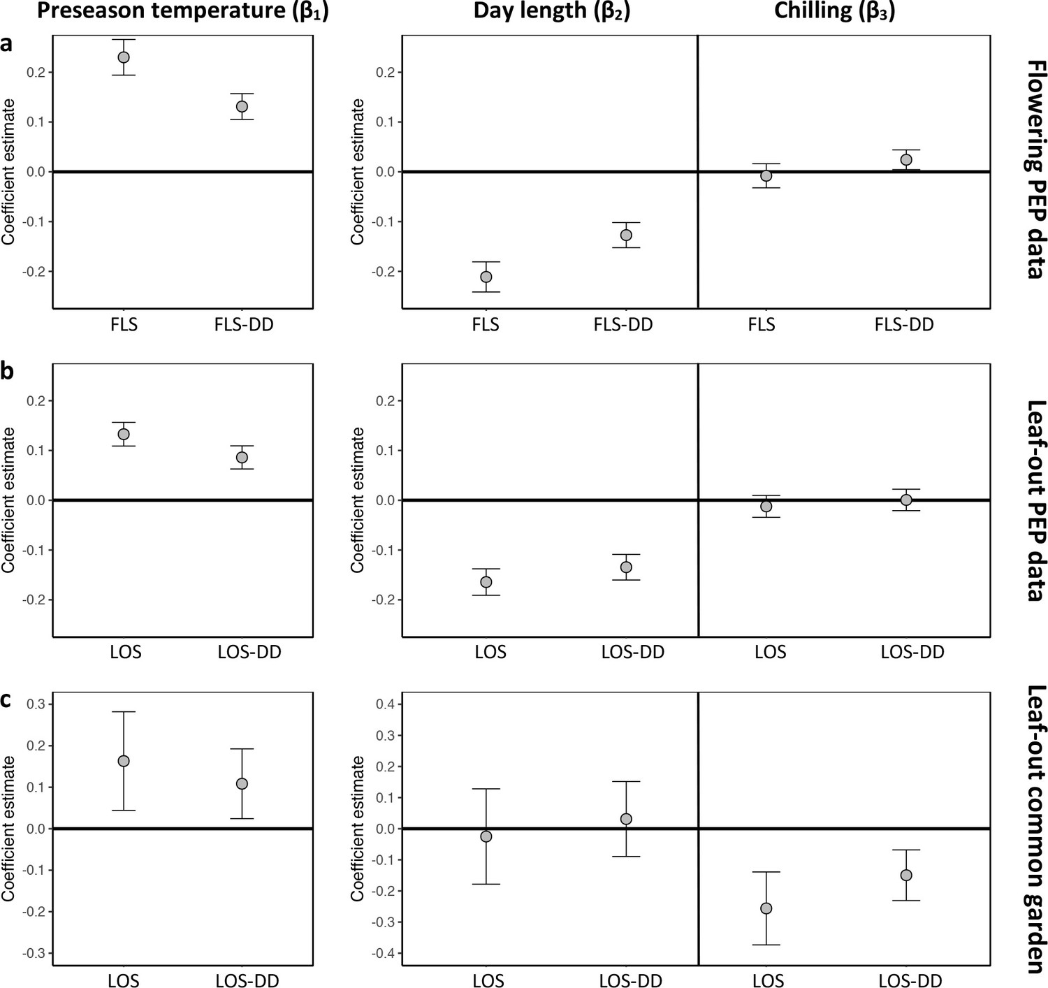
Hierarchical Bayesian models to test for the environmental drivers of inter- individual flowering (a) and leaf-out (b, c) synchrony.

Plots show coefficient values (β) [means and 95% credible intervals] for equations 6 and 7 (see Materials and methods). PEP data (a, b) or common-garden observations (c) were used for analysis. Left panels: The effect of preseason temperature on inter-individual phenological synchrony measured either as the standard deviation in leaf-out/flowering dates (LOS/FLS) or the standard deviation in degree-day (DD) requirements among individuals (LOS-DD/FLS DD). Right panels: The effects of day length and winter chilling on inter-individual leaf-out synchrony. To account for within-species rather than among-species synchrony, all models include species random effects. The models using the PEP data (a and b) additionally include site random effects (1° pixels) to address within-pixel phenological synchrony. All variables were standardized to allow for direct effect size comparisons. N = 13 (a), 9 (b), and 59 species (c).

https://doi.org/10.7554/eLife.40214.008

Which factors cause the loss of inter-individual synchrony under climate warming? One possibility is that individuals reach their forcing sums (accumulated warming required for leaf-out or flowering) over a longer period because ‘within-spring warming speed’ may be decreasing, flattening the temperature curve during spring (Wang et al., 2015; Wang et al., 2016). Thus, while the time span among individual leaf-out times might increase, differences in the forcing sums required until leaf-out or flowering among individuals might remain similar (Figure 2—figure supplement 2a). To test this, we additionally calculated leaf-out/flowering synchrony as the standard deviation in individual forcing requirements (degree-days [DD] from 1 January until leaf-out/flowering) [hereafter referred to as LOS-DD and FLS-DD] for both the PEP and Munich common garden data. In both data sets, we found a strong (albeit slightly weaker compared to the LOS/FLS analysis) negative relationship between preseason temperature and LOS-DD, that is, individual differences in the forcing sums required until leaf-out or flowering are increasing with warmer preseasons (Figure 2a and Figure 2—figure supplement 1). We also simulated synchrony of spring phenology based on the Munich Jan–May temperatures over the past 60 years, assuming that phenology is solely driven by degree-day accumulation (no effect of day length or winter chilling; see Figure 2—figure supplement 2b). This simulation revealed losses of synchrony under warmer preseasons (regression coefficients between 0.15 and 0.43 SD/°C; Figure 2—figure supplement 2c), but those simulated losses are small relative to the actual losses inferred from in situ observations (see red arrows in Figure 1—figure supplement 1a and Figure 1—figure supplement 2a). Together, those results show that a flattening temperature curve during spring is not sufficient to explain the declining inter-individual synchrony in the 72 species analyzed here.

Warmer preseasons in spring are associated with both reduced accumulation of winter chilling and shorter day-lengths at spring onset, and previous experiments on plant phenological strategies have shown pronounced differences among species in their reactions to day length and winter chilling (Zohner et al., 2017; Laube et al., 2014; Zohner et al., 2016). To test whether similar differences within species might explain the decrease in LOS and FLS under climate warming detected in our in-situ data, we designed experiments in which we exposed trees to different regimes of spring warming, winter chilling, and day length. We additionally tested for the relative effects of winter chilling and day length on LOS and FLS using the PEP and Munich common garden data (for each year and individual, we calculated winter chilling experienced until leaf-out and day length for the date when an individual’s average forcing requirement had been reached).

A first experiment addressed inter-individual variation in spring warming (‘forcing’), day length, and winter chilling requirements in 11 mature Fagus sylvatica trees growing in the vicinity of the botanical garden in Munich. Twigs were cut at three dormancy stages during winter and exposed to different day-length regimes (8 hr, 12 hr, or 16 hr light per day) and ambient spring-forcing conditions (mean daily temperature of 16°C). Note that in beech, leaf-out and flowering occur simultaneously because leaves and flowers are located on the same preformed shoots within overwintering buds. The results showed large differences in forcing and day-length requirements among individuals (Figure 3a and b): for example, while in individual 1, day length had no effect on the amount of warming required until leaf-out, in individual 11, warming requirements were >2 x lower under long-day than under short-day conditions (Figure 3b). Chilling requirements differed little among individuals (compare slopes in Figure 3c).

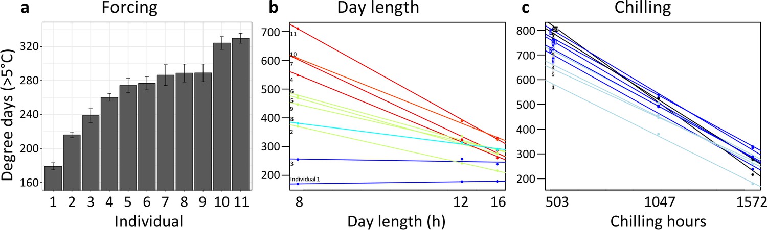
Individual differences in the forcing (a), day-length (b), and chilling (c) requirements among 11 beech trees (F. sylvatica; Experiment 1).

(a) Mean ( ± SEM) forcing requirements (accumulative degree-days >5°C) until leaf-out under long chilling and constant 16 h day length. (b) Degree-days until leaf-out at 8 hr, 12 hr, and 16 h day length (collection date: 21 March 2015). Colours according to slope (red: steep slope; blue: no slope). (c) Degree-days until leaf-out under short, intermediate, and long chilling (collection dates: 22 Dec 2014, 6 Feb 2015, 21 March 2015) and 16 h day length. Colours according to slope (dark blue: steep slope; light blue: no slope).

https://doi.org/10.7554/eLife.40214.011

In a second experiment, we cut twigs of the same 11 beech trees at eight dormancy stages during winter and exposed them to natural day length. Temperatures were the same as in experiment 1, that is, ambient. This allowed us to determine (i) the extent to which differential reliance on forcing, day length, and winter chilling (as inferred from experiment 1) explains LOS/FLS under natural light conditions, and (ii) the effect of warmer winter and spring conditions on LOS/FLS. Leaf-out variation among individuals explained most of the total variation among twigs, with 52% attributable to between-individual variation, 33% to treatments, and only 15% to within-individual variation (Figure 4—figure supplement 1). As in the in situ data from the Pan European Phenology network, synchrony strongly decreased under warmer spring conditions (Figure 4a,b). We hypothesized that differences in day-length sensitivity among individuals (as documented for F. sylvatica; Figure 3b) can explain this: Under cold winter conditions, days are already long when spring warming occurs, reducing the effect of a tree’s day length sensitivity on its leaf-out time, whereas with early spring warming, days are still short, preventing day-length sensitive trees from flushing. In natural populations, leaf-out advancement in day length-sensitive individuals, but not in day length-insensitive individuals, will thus increase the period of leaf-out under short day conditions. Both the experimental and the PEP in situ data confirm this idea, showing that (i) phenological synchrony among individuals strongly decreases under short day conditions (Figures 2b and 3b) and (ii) differences in day-length requirements are the single most important factor explaining individual variation in leaf-out times (Figure 4c,d).

Figure 4 with 1 supplement see all
Loss of phenological synchrony with climate warming is explained by contrasting day-length sensitivities in Fagus sylvatica.a, b, Experiment 2.

(a) Leaf-out dates of Fagus sylvatica (blue), Fagus crenata (dotted grey), and Quercus robur (grey) under varying winter lengths (chilling hours = sum of hours from 1 November until leaf-out with an average temperature between 0°C and 5°C). Bars show the standard deviation of average leaf-out dates among 11 F. sylvatica individuals. The shaded area shows the difference between the leaf-out date of the first flushing twig of the first individual and the last twig of the last individual to leaf- out, using a LOESS smoothing function. For F. crenata and Q. robur, we investigated one individual each and therefore do not report inter-individual variation. (b) Standard deviation of leaf-out dates among 11 F. sylvatica individuals at different winter lengths (chilling levels) and natural day length. (c) The effect of individual day-length sensitivity on the timing of leaf unfolding when twigs were collected on 10 December 2015. Note the reversed x-axis scale, that is, smaller values indicate higher day-length sensitivity. (d) Variables explaining the sequence of leaf-out dates of 11 F. sylvatica individuals at eight different chilling levels. The percentage of leaf-out variation (derived from the ANOVA sums of squares) that can be explained by individual forcing requirements (red), day-length requirements (green), chilling requirements (blue), and the remaining residuals, that is, unexplained variation (black). *p<0.05; **p<0.01; ***p<0.001.

https://doi.org/10.7554/eLife.40214.012

This insight explains why, especially in Fagus sylvatica, in which day length has the most pronounced effect on spring phenology (Laube et al., 2014; Zohner et al., 2016), LOS is strongly affected by preseason temperatures (Figure 1c). By contrast, in day-length insensitive species, such as silver birch Betula pendula and Norway spruce Picea abies (Zohner et al., 2016), preseason warming has a smaller (but still significant) effect on LOS, suggesting that heritable differences in day-length sensitivity are a major driver of phenological variation among individuals. In our common garden data, the standard deviation of inter-individual leaf-out times increased by 0.09 ± 0.02 (mean ± CI) days per decrease in one chilling day, and the standard deviation of inter-individual forcing requirements increased by 0.23 ± 0.06 degree-days per decrease in one chilling day (lower panel Figure 2b), indicating that individual differences in the sensitivity to winter chilling also contribute to the observed loss of phenological synchrony under climate warming.

What biological consequences can be expected from less synchronized leaf-out and flowering of the individuals of a species? With regard to vegetative development, precocious leaf unfolding under warm springs increases the risk of late frost damage (Augspurger, 2013; Kollas et al., 2014; Vitasse et al., 2014), but also potential carbon gain due to earlier photosynthetic activity (Keenan et al., 2014). This risk-return trade-off will affect selection on suitable genotypes under future conditions, and the increasing spread of leaf-out should increase the selective importance of spring phenology. Whether opportunistic phenological strategies (relying on temperature as the main trigger) or conservative strategies (relying on day length and/or winter chilling as a buffer against highly variable spring temperatures) will be favored in the future will be region-specific, depending on the relative advancement rates of spring warming and late frost events. In continental regions, where the advent of spring is relatively invariable (low late frost risk), phenological strategies reliant on temperature should be favored (Zohner et al., 2017; Körner and Basler, 2010).

With regard to flowering, decreased synchrony among individuals, as already strongly evident in Alnus glutinosa (Figure 1f), should lead to reduced inter-individual pollen transfer. Strong divergence in flowering times among individuals also might lead to assortative mating (depending on incompatibility systems), possibly promoting local adaptation (Antonovics and Bradshaw, 1970; Kirkpatrick, 2000; Weis and Kossler, 2004) and should act as a buffer against climate change-induced phenological mismatch between plants and leaf-feeding or pollen-collecting insects (Renner and Zohner, 2018). Rapid adaptive responses, for instance a filtering out of extreme phenotypes through increased mortality or reduced reproduction, might counteract warming-induced losses of inter-individual synchrony. Such selection of the standing variation can occur very rapidly, at least in herbaceous plants (Jump and Penuelas, 2005; Fakheran et al., 2010).

While our results show that climate warming causes a loss of phenological synchrony among the individuals of a population, a study of leaf-out along elevational gradients in four European tree species, between 1960 – 2016, revealed that leaf-out times at higher and lower elevations are today compressed into a shorter time window compared to 58 years ago (Vitasse et al., 2018). These findings do not contradict those of the present study because populations growing at high elevations were able to advance their phenology more than those at lower elevations for which chilling and/or day-length requirements are no longer fulfilled (Figure 5). As a result, the leaf-out times of high- and low-elevation populations are converging (Vitasse et al., 2018). At the same time, however, differences in day-length sensitivity (as well as chilling and temperature sensitivity) among the individuals at any one elevation under climate warming are resulting in diverging flowering and leaf-out times within populations. A likely side-effect of increasing phenological variation within populations is a community-level reduction of variation between species, which could reduce phenological niche differentiation between species and alter competitive environments (CaraDonna et al., 2014).

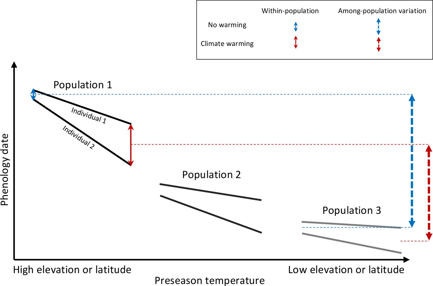
Schematic representation of within- and among-population phenological synchrony in response to climate warming.

As demonstrated in this study, inter-individual synchrony within a population will decrease under warmer preseason temperatures because individuals differ in their sensitivity to temperature. Within-population variation under ambient or warmed preseason temperatures is illustrated by the solid blue and red arrows, respectively. By contrast, phenological synchrony among populations is expected to increase, given that populations in warm regions (Population 3) will advance their phenology less than populations in cold regions (Population 1). This is illustrated by the dashed blue and red arrows, showing that the difference in the average phenological date between Population 1 and 3 is smaller under warmer preseasons (red dashed arrow) than under ambient preseason temperatures (blue dashed arrow).

https://doi.org/10.7554/eLife.40214.014

The overall prediction from the present findings is that human-caused climate warming is leading to plant phenologies that are more heterogeneous within populations and more uniform among populations (over altitude or latitude) and among species (within communities). The rapid loss of reproductive and vegetative synchrony in European plant populations also predicts changes in their gene flow and trophic interactions, although community-wide consequences are presently unknown.

Conclusion

The synchrony of developmental stages among organisms is a critical aspect of ecosystem functioning. Here, based on ground observations and climate-manipulation experiments, we show that global warming is altering within-population synchrony of leaf-out and flowering dates in temperate plants, with warmer temperatures reducing inter-individual synchrony by up to 55%. Experiments suggest that individual differences in the sensitivity to day-length and/or winter chilling underlie the loss of synchrony, and future climate warming is expected to further strengthen this trend. These results predict consequences for gene flow and trophic interactions, but also emphasize the importance of adaptation when forecasting future plant growth and productivity.

Materials and methods

Analysis of leaf-out and flowering synchrony (LOS and FLS) using the PEP database

Data sets

Request a detailed protocol

In situ phenological observations were obtained from the Pan European Phenology network (Templ et al., 2018), which provides open-access European phenological data. Leaf-out dates were analyzed for nine species, flowering dates for 15. Data from Germany, Austria, and Switzerland were used for the analysis. For the angiosperm woody species, leaf-out was defined as the date when unfolded leaves, pushed out all the way to the petiole, were visible on the respective individual (BBCH 11, Biologische Bundesanstalt, Bundessortenamt und Chemische Industrie). For the two conifers Larix decidua and Picea abies, leaf-out was defined as the date when the first needles started to separate (‘mouse-ear stage’; BBCH 10). Flowering was defined as the date of beginning of flowering (BBCH 60). We removed (i) individual time series, for which the standard deviation of phenological observations across years was higher than 25 and (ii) leaf-out and flowering dates that deviated from an individual’s median more than three times the median absolute deviation (moderately conservative threshold) (Vitasse et al., 2018). Here, we consider time series as being equal to individuals because, in the PEP database, the same individual is usually observed for many years. However, we acknowledge that this does not necessarily have to be the case for all time series, as individuals might die or not be detectable due to other reasons.

Analysis

To test for an effect of spring temperature on inter-individual leaf-out synchrony (LOS) and flowering synchrony (FLS), we divided the study area into pixels of one degree resolution (~110×85 km), an area that can reasonably be considered as reflecting populations, at least for wind-pollinated woody species (see discussion on herbs in the main text). To allow for within-pixel comparisons of LOS and FLS between years, data from the same individuals had to be used each year. To achieve this, we kept only pixels for which there were at least three individuals with data for the same 15 years. For each pixel, we deleted all (i) individuals growing at altitudes that deviated by >200 m from the average altitude of all individuals within the pixel, and (ii) years that had less than 90% plant-coverage, that is, data from at least 90% of the individuals within the pixel had to be available for the respective year, otherwise the year was excluded from the analysis. This data cleaning left us with a total of 12,536 individuals, 317,672 phenological observations (individuals x year), and a median time-series length of 25 years (minimally 15 years, maximally 48 years). The number of individuals within pixels (per species and phenological stage) ranged between 3 and 53 (median = 12). See Figure 1—figure supplement 1b and Figure 1—figure supplement 2b for information on the number of pixels used per species.

For each year and species, LOS and FLS within pixels were then calculated as the standard deviation of leaf-out or flowering dates. Additionally, we calculated the standard deviation of forcing requirements among individuals (subsequently referred to as LOS-DD [leaf-out synchrony degree-days] and FLS-DD [flowering synchrony degree-days]) to test if greater phenological variation among individuals can be explained by increasing variation in forcing requirements. Individual forcing requirements until leaf-out were calculated as the sum of degree-days (DD) from 1 January until leaf-out or flowering using 5°C as base temperature (e.g., Zohner and Renner, 2015):

DDsumt= totLOTt-5

where DDsum is the accumulated degree days until leaf unfolding, tLO is the day of leaf unfolding, Tt is the mean daily temperature on day t, and t0 is the start date for forcing accumulation, which was fixed at 1 January. For each year and species, LOS-DD and FLS-DD within pixels were then calculated as the standard deviation of forcing requirements until leaf-out or flowering dates.

The daily mean air temperature at each site was derived from a gridded climatic data set of daily mean temperature at 0.5° spatial resolution (approximately 50 km, ERA-WATCH) (Beer et al., 2014). For each year, preseason temperature within pixels was defined as the average temperature during the 60 days prior to the average leaf unfolding or flowering date within the respective pixel, which is the period for which the correlation coefficient between phenological event and temperature is highest (Fu et al., 2015).

To test if shortened day lengths or reduced winter chilling explain the decrease in phenological synchrony under warmer preseasons, for each year, pixel, and species, we calculated the average chilling hours until leaf-out or flowering and the average day length (DL) at the date (DOY) when the average forcing requirements until leaf-out or flowering were fulfilled. Chilling hours were calculated on basis of 6-hourly temperature data (CRU-NCEP, spatial resolution of 0.5°; https://crudata.uea.ac.uk/cru/data/ncep/), as the sum of hours from 1 November until leaf-out/flowering with an average temperature between 0°C and 5°C (e.g., Vitasse et al., 2018):

(1) Chsum(t)= totLO1 if 0Tt5

where Chsum is the sum of chilling hours until leaf unfolding, tLO is the day of leaf unfolding, Tt is the hourly mean temperature on hour t, and t0 is the start date for chilling accumulation, which was fixed at 1 November in the year before leaf unfolding.

DL was calculated as a function of latitude and DOY (Forsythe et al., 1995):

(2) DL=2424πcos1[ sin0.8333π180+sinLπ180sinφcosLπ180cosφ]
(3) φ=sin1(0.29795cosθ)
(4) θ=0.2163108+2tan1(0.9671396tan(0.0086(DOY186)))

where L is the latitude of the phenological site.

Statistical analyses

Request a detailed protocol

Within each pixel we applied linear models to test for an effect of preseason temperature, day length, and winter chilling on phenological synchrony (LOS, LOS-DD, FLS and FLS-DD). We then determined the frequency distributions for the correlation coefficients between phenological synchrony and preseason temperature across all species and sites. For each species, we applied t-tests to detect whether the average of all correlation coefficients obtained for each pixel differs from zero. To model changes in the distribution of within-pixel leaf-out and flowering dates (means and standard deviations) in response to temperature, we applied mixed-effects models using average leaf-out/flowering dates or LOS/FLS as response variables, preseason temperature as explanatory variable, and site as a random effect to control for the use of different sites in the model.

Additionally, we applied a hierarchical Bayesian model to test for the relative effects of preseason temperature, winter chilling, or day-length on (i) inter-individual variation in leaf-out/flowering date (LOS / FLS) and (ii) inter-individual variation in forcing requirements until leaf-out/flowering (LOS-DD / FLS-DD). The use of a Bayesian framework allowed us to fit slope parameters across traits simultaneously without concerns of multiple testing or P-value correction. All models included random intercept effects for (i) species (to address within-species rather than between species phenological synchrony) and (ii) pixels (to address within-pixel rather than between-pixel phenological synchrony). Our model includes four dependent continuous variables (LOS, LOS-DD, FLS, and FLS-DD) that are normally distributed with mean µ, varianceσ2, and correlation structure Σ, hereafter referred to as dependent:

(5) dependentiN(μdependent i,σ2, Σ)

Regression components of the model are of the form:

(6) μdependent i=α1+β1×preseason tmpi+speciesi+pixeli
(7) μdependent i=α1+β2×daylengthi+β3×chillingi+speciesi+pixeli

where the term α refers to the intercept, β to the estimated slopes of the respective variable in Figure 2, and dependent refers to synchrony values (i) [LOS, LOS-DD, FLS, or FLS-DD]. To allow for direct effect size comparisons, all continuous variables were standardized by subtracting their mean and dividing by 2 SD before analysis (Gelman and Hill, 2007). The resulting posterior distributions are a direct statement of the probability of our hypothesized relationships. Effective posterior means ± 95% confidence intervals are shown in Figure 2.

To parameterize our models, we used the JAGS implementation (Plummer, 2003) of Markov chain Monte Carlo methods in the R package R2JAGS (Y-S and Yajima, 2014). We ran three parallel MCMC chains for 200,000 iterations with a 50,000-iteration burn-in and evaluated model convergence with the Gelman and Rubin (Gelman and Rubin, 1992) statistic. Noninformative priors were specified for all parameter distributions, including normal priors for α and β coefficients (fixed effects; mean = 0; variance = 1,000), and uniform priors between 0 and 100 for the variance of the random intercept effects, based on de Villemereuil and colleagues (de Villemereuil et al., 2012). All statistical analyses relied on R 3.2.2(R Core Team, 2018).

Analysis of leaf-out synchrony (LOS) using common-garden data from 2013 to 2018

Request a detailed protocol

Between 2013 and 2018 we observed the leaf-out dates of 209 individuals in 59 temperate woody species (minimally three individuals per species) in the Munich Botanical garden (see Supplementary Materials Supplementary file 1 for a list of species). An individual was scored as having leafed out when at least three branches had unfolded leaves pushed out all the way to the petiole (International Phenological Gardens of Europe, 2017). To test whether the trends observed in the PEP analysis are consistent with our common garden data, the same parameters (LOS, LOS-DD, preseason temperature, winter chilling, and day length) were calculated as described above (Analysis of leaf-out and flowering synchrony (LOS and FLS) using the PEP database). We then applied hierarchical Bayesian models including species random effects (see paragraph above) to test for the effects of preseason temperature, winter chilling, and day-length on LOS and LOS-DD.

Twig cutting experiments and phenological scoring

Request a detailed protocol

To study the extent of intraspecific variation in leaf-out strategy (within-species variation in day length, chilling, and forcing requirements) and its implications under climate warming, we conducted twig-cutting experiments on mature Fagus sylvatica individuals growin in the vicinity of Munich. Experiments have demonstrated that twig cuttings precisely mirror the phenological behavior of their donor plants and therefore are adequate proxies for inferring phenological responses of adult trees to climatic changes (Zohner and Renner, 2015; Vitasse and Basler, 2014). We used twigs approximately 50 cm in length, and immediately after cutting, we disinfected the cut section with sodium hypochlorite solution (200 ppm active chlorine), cut the twigs a second time, and then placed them in 0.5 l glass bottles filled with 0.4 l cool tap water enriched with the broad-spectrum antibiotics gentamicin sulfate (40 μg l−1; Sigma-Aldrich, Germany) (Zohner et al., 2016; Zohner and Renner, 2015). We then transferred the cut twigs to climate chambers and kept them under short (8 hr), intermediate (12 hr), or long day (16 hr) conditions (see Experiment one below), or natural day length (Experiment two below). Temperatures in the climate chambers were held at 12°C during the night and 20°C during the day, with an average daily temperature of 16°C to simulate forcing temperatures. Illuminance in the chambers was about eight klux (∼100 μmol s−1 m−2). Relative air humidity was held between 40% and 60%. To account for within-individual variation, we used 10 replicate twigs per individual treatment and monitored bud development every second day. For each individual and treatment, we then calculated the mean leaf-out date out of the first eight twigs that leafed out. A twig was scored as having leafed out when three buds had unfolded leaves pushed out all the way to the petiole (International Phenological Gardens of Europe, 2017). Forcing requirements until leaf-out were calculated as the sum of degree-days [outside of and in climate chambers] from 10 December (1st collection date) until leaf-out using 5°C as base temperature (e.g., Zohner and Renner, 2015). Chilling hours were calculated as the sum of hours from 1 November until leaf-out with an average temperature between 0°C and 5°C.

Experiment 1: Differences in day length sensitivity among Fagus sylvatica individuals

Request a detailed protocol

In winter 2014/2015, twigs of 11 individuals (10 replicate twigs per individual and treatment) of Fagus sylvatica were collected at three dates during winter (22 Dec 2014, 6 Feb 2015, and 21 Mar 2015) and brought into climate chambers. Additionally, we collected twigs from one individual each of Fagus crenata and Quercus robur. Temperatures in the chambers ranged from 12°C during night to 20°C during day, with an average daily temperature of 16°C. Day length in the chambers was set to 8 hr, 12 hr, or 16 hr.

Individual day length sensitivity was defined as the slope of the function between day-length treatment and accumulated degree days (>5°C) until leaf-out (twigs were collected on 21 March; see Figure 3b). The steeper the slope, the stronger the effect of day length on the amount of warming required for leaf-out. A flat slope indicates that day length has no effect on the timing of leaf-out.

Individual chilling sensitivity was defined as the slope of the function between chilling treatment (collection date) and accumulated degree days (>5°C) until leaf-out when twigs were kept under constant 16 h day length (see Figure 3c). The steeper the slope, the stronger the effect of chilling on the amount of warming required for leaf-out.

Individual forcing requirement was defined as the accumulated degree days (>5°C) until leaf-out under long chilling (21 March collection) and constant 16 h day length (see Figure 3a). Under such conditions, chilling requirements and day length requirements should be largely met, and thus the remaining variation in leaf-out dates should be largely attributable to differences in forcing (warming) requirements.

Experiment 2: Different reactions to climate warming among Fagus sylvatica individuals

Request a detailed protocol

In winter 2015/2016, twigs from the same 11 individuals were harvested every two weeks (from 10 December until 21 March) and kept under the same temperature conditions applied in experiment 1 (12°C during night to 20°C during day), with natural day length. This allowed us to test if those individuals with no/little day length sensitivity would advance their leaf-out more under short winter conditions than day length-sensitive individuals, and to determine the relative effect of individual variation in day length requirements, chilling requirements and forcing requirements on leaf-out variation under different winter/spring conditions (Figure 4). Within-species leaf-out synchrony (LOS) was calculated as the standard deviation of individual leaf-out dates. To analyze which leaf-out cues (day length, chilling, and forcing requirements) best explain leaf-out variation among individuals, we applied a multivariate linear model, including individual forcing, day length, and chilling requirements (as inferred from experiment 1) as explanatory variables. To express the total variation in leaf-out dates that can be attributed to each trait, we used ANOVA sums of squares (see Figure 4d).

To infer which percentage of the variation in leaf-out dates is due to treatment effects, between-individual variation, or within-individual variation, we calculated variance components by applying a random-effects-only model including treatments and individuals as random effects (individuals nested within treatments) (Figure 4—figure supplement 1).

Data availability

All data generated during this study are included in the manuscript and supporting files. The in situ phenological data we analyzed can be found here following the creation of a free account: http://www.pep725.eu/data_download/data_selection.php

References

    1. Chuine I
    2. Beaubien E
    (2001)
    Phenology is a Major determinant of temperate tree range
    Ecology Letters 4:500–510.
    1. Chuine I
    (2010) Why does phenology drive species distribution?
    Philosophical Transactions of the Royal Society B: Biological Sciences 365:3149–3160.
    https://doi.org/10.1098/rstb.2010.0142
  1. Book
    1. Gelman A
    2. Hill J
    (2007)
    Data analysis using regression and multilevel/hierarchical models
    Cambridge, UK: Cambridge University Press.
    1. Kirkpatrick M
    (2000) Reinforcement and divergence under assortative mating
    Proceedings of the Royal Society B: Biological Sciences 267:1649–1655.
    https://doi.org/10.1098/rspb.2000.1191
  2. Conference
    1. Plummer M
    (2003)
    JAGS: a program for analysis of bayesian graphical models using gibbs sampling
    Proceedings of the 3rd International Workshop on Distributed Statistical Computing 2003.
  3. Software
    1. R Core Team
    (2018)
    R: a language and environment for statistical computing
    R Foundation for Statistical Computing, Vienna.
  4. Software
    1. Y-S S
    2. Yajima M
    (2014)
    R2jags: a package for running JAGS from R
    R Package Version.

Decision letter

  1. Bernhard Schmid
    Reviewing Editor; University of Zurich, Switzerland
  2. Ian T Baldwin
    Senior Editor; Max Planck Institute for Chemical Ecology, Germany

In the interests of transparency, eLife includes the editorial decision letter, peer reviews, and accompanying author responses.

[Editorial note: This article has been through an editorial process in which the authors decide how to respond to the issues raised during peer review. The Reviewing Editor's assessment is that all the issues have been addressed.]

Thank you for submitting your article "Loss of leaf-out and flowering synchrony under global warming" for consideration by eLife. Your article has been reviewed by three peer reviewers, including Bernhard Schmid as the Reviewing Editor and Reviewer #1, and the evaluation has been overseen by Ian Baldwin as the Senior Editor. The following individual involved in review of your submission has agreed to reveal their identity: Kentaro K Shimizu (Reviewer #2). A third reviewer remains anonymous.

The Reviewing Editor has highlighted the concerns that require revision and/or responses, and we have included the separate reviews below for your consideration. If you have any questions, please do not hesitate to contact us.

Summary:

This paper shows that increased pre-growing-season temperatures in central Europe lead to a wider spread of leaf-out and flowering-start days among individuals in several tree and other plant species. The potential causes – in particular within-population variation in preseason-temperature, photoperiod and chilling degree-day requirements – are analyzed. In addition, the slower increase in temperature in spring with increasing overall temperatures plays a role in the reduced synchrony of phenological events within species. The authors discuss potential consequences, i.e. reduced genetic exchange between individuals due to different flowering times and altered interactions with herbivores due to different leaf-out times.

Major concerns:

These are pointed out in the reviews below. In particular, please:

- discuss the issue of within- vs. between-species asynchrony/synchrony;

- justify the choice of 60 days preseason interval;

- improve figure explanations;

- be careful with the use of the term "genetic", acknowledge other sources of variation;

- mention caveats such as masting, beech as extreme case, experimental focus on photoperiod;

- replace population by grid-cell or find other solution for the problem mentioned by the third reviewer;

- explain more clearly the nature of extracted data (site- or individual-level?) and the statistical analysis used for each data set;

- consider the additional references mentioned below.

Separate reviews (please respond to each point):

Reviewer #1:

This paper shows that increased pre-growing-season temperatures in central Europe lead to a wider spread of leaf-out and flowering-start days among individuals in several tree and other plant species. The potential causes – in particular within-population variation in preseason-temperature, photoperiod and chilling degree-day requirements – are analyzed. In addition, the slower increase in temperature in spring with increasing overall temperatures plays a role in the reduced synchrony of phenological events within species.

The authors discuss potential consequences, i.e. reduced genetic exchange between individuals due to different flowering times and altered interactions with herbivores due to different leaf-out times. The increased within-population variation will also reduce the between-population variation across sites. Additionally, but not discussed by the authors, it may reduce between-species variation within sites, which could affect niche separation between species and thus potential biodiversity effects on pollinators and herbivores.

Generally, this paper is very comprehensive, as it uses different sources of evidence, including experiments, and careful analyses of data. It describes previously unknown phenomena for a representative set of plant species and analyzes underlying causes. Thus, I have only two major points that in my view need clarification:

1) In several places the authors refer to synchrony between species to derive or justify that here they looked at synchrony within populations. However, I think the logic is not as sound as it could be. In particular, if they do want to make a link between the two levels, they should rather discuss the potential anti-correlation mentioned above, i.e. that a loss of phenological "specialization" (synchrony) of species will lead to more overlap (synchrony) between species at community level. I understand that the authors did not directly analyze the latter because their species were not selected randomly within pixels, but at least a discussion would be useful (or they might even have some data to do the analysis, because for that species with less complete data could also be included).

2) An important assumption in the analysis of effects of pre-season temperature is that the time of 60 days before leaf unfolding or flowering start is the correct one. It would be important to know if other time intervals would have led to similar results, as currently it looks quite arbitrary why 60 days should be best. Such an analysis of different pre-season intervals could be added to the supplement.

The following minor comments are given:

Abstract: delete "genetic".

Delete "Such species-specific responses imply variation in heritable phenological strategies among individuals,".

Introduction, first paragraph: "foliovores"?

Introduction, second paragraph: "common-garden".

Results and Discussion, third paragraph: delete "Surprisingly,".

Results and Discussion, third and fourth paragraphs: "increased".

Results and Discussion, fourth paragraph: LOS and FLS could be analyzed together as in multivariate anova. Just put the two data tables vertically together and add a column "trait".

Results and Discussion, twelfth paragraph: a further useful citation here would be Fakheran et al., 2010.

Results and Discussion, last paragraph: here you may refer to other papers showing "biotic homogenization" due to global change.

Results and Discussion, last paragraph: delete "massive".

Materials and methods subsection “Analysis”, fourth paragraph: delete "and/".

Additional data files and statistical comments:

The statistical analysis is sound. Species identity was used as random term – specific species responses could have been analyzed in more detail with species identity or contrasts thereof as fixed term(s).

Reviewer #2:

The effect of temperature change on phenology has attracted a lot of attentions, and many studies reported the change in the timing of plant phenological events. The authors focused on the variation in a population, or synchrony of leaf-out and flowering. Curiously, they found that plant synchrony is low in years with high temperature in temperate forests. They combined evidence of a long-term survey, transplantation and manipulation experiments. The manuscript addressed important questions and reported novel findings.

I have a few comments on the way of presentation of the figures.

First, the figure numbers are often not ordered in number. Please check throughout the manuscript. For example, in the Results and Discussion, Figure 1—figure supplements 4 and 5 appeared in the fourth paragraph, then Figure 2—figure supplement 1, Figure 2—figure supplement 2B, Figure 2—figure supplement 2CFigure in the sixth paragraph, nothing on Figure 2—figure supplement 2A. Figure 4—figure supplement 1 was mentioned at the last sentence of the Materials and methods, but it should be mentioned as Results. The legend of Figure 1—figure supplements 1 and 2 said "Extended Data Figure 5", which does not exist. Figure 1C and D appeared before 1A and B, which may depend on the style of the journal. These are likely remnants of a previous version of the manuscript.

More importantly, how to interpret figures are often not well explained in the main text or figure legends. If a reader reads carefully throughout the manuscript, one may find the logics, but they should be clarified in the main text. "We also simulated synchrony of spring phenology based on the Munich Jan-May temperatures over the past 60 years, assuming that phenology is solely driven by degree-day accumulation (no effect of photoperiod or winter chilling; see Figure 2—figure supplement 2B) and this simulation revealed small losses of synchrony (R2 values between 0.04 and 0.11 and regression coefficients between 0.15 and 0.43, see Figure 2—figure supplement 2C)."

It is not self-evident how Figure 2—figure supplement 2B and C supported these conclusions. To conclude "small", what did you compare with?

Figures"(i) phenological variation among individualsstrongly decreases under short day conditions (Figures 2B and 3B))." It is not self-evident how these figures supported this conclusion. Figure 2B does not show short day directly (photoperiod is there). In Figure 3B, at a first glance, the variation appears high at short day (8-hour day length).

Results and Discussion, ninth paragraph. I would suggest to remove the term "genetic" differences among individuals. I agree that the data suggest most likely, but other possibilities cannot be excluded. For example, plant age or size may affect the temperature responses.

Manipulation and transplantation experiments

Describe more about the nature of the used trees of the manipulation experiments as well as of transplantation experiments. Are they more or less natural trees or from the same region? Genetic data would be the best if any, but historical description would be valuable. In a botanical garden, some of the trees may be transplanted from distant populations. Non-local plants may react to environmental changes differently. Even so, the data supports the individual differences, but it may not support the increase of variation in a small geographic scale.

Some tree species may show masting and may affect the analysis, but it was not clearly mentioned in the text. For masting species, was there no flowering in some years, or did they still flower every year to some extent? Particularly, there are number of studies on the meteorological factors and nutritional effect on the masting of Fagus sylvatica and F. crenata, two of the species studied in this manuscript (for example, Overgaard et al., 2007 Effects of weather conditions on mast year frequency in beech (Fagus sylvatica L.) in Sweden. Forestry, 80, 555-565; Miyazaki et al. 2014 Nitrogen as a key regulator of flowering in Fagus crenata: understanding the physiological mechanism of masting by gene expression analysis. Ecol Lett 17, 1299-1309.)

Minor Comments:

Results and Discussion, sixth paragraph: define forcing sums clearly.

Results and Discussion, ninth paragraph: it was not clear if this is a hypothesis or results. By reading later sentences, this seems a hypothesis. Please clarify it.

Legend of Figure 2—figure supplement 1: B is bold but C is not.

Reviewer #3:

"Loss of leafout and flowering synchrony under global warming" is an interesting paper on an important topic. The authors have combined long-term data from PEP725 (an impressive database, used for decades in the field) with observations from an arboretum and experiments on Fagus sylvatica (henceforth European beech) to attempt to measure changes with climate change in 'within-population' synchrony of leafout and flowering for a handful of species, and then attribute the changes to primarily genetic differences across individuals in photoperiod responses.

Many papers have previously highlighted the potentially increasing importance of genetic variation in phenology with climate change altering the environmental playing field. The paper offers two (I believe new) experiments on European beech, which are an important contribution to the field of phenology.

Unfortunately the paper also suffers from several major flaws that prevent it from having the impact I think it could. I outline these below in no particular order:

1) The authors choose to do experiments on European beech to test their hypothesis that individual variation in predominantly photoperiod responses lead to observed variation in synchrony. Decades of research have highlighted that European beech has the most extreme responses to photoperiod of any species studied, which the authors do not clearly acknowledge.

2) The authors' experiments are ideally designed to test for photoperiod differences. This is because photoperiod is the only factor they fully vary in their experiments (they partially manipulate chilling by taking cuttings across time and their forcing temperatures are always ambient). This means the authors have designed their experiment to maximize differences observed in photoperiod responses, and minimized the potential to find forcing (or chilling) differences.

(*) Pts 1 and 2 taken together mean the most novel parts of the paper were predisposed to find very strong photoperiod effects, and this reality should temper any strong conclusions regarding photoperiod in relation to other cues that are drawn from this paper. I think the paper would be stronger if the authors would acknowledge this more clearly.

3) The authors claim to make conclusions about 'populations' but they don't fully define a population. It is defined for PEP725 data and in this case it's a one-degree gridcell. They toss out some PEP725 data based on deviation in altitude or data deemed too variable but I doubt this helps them achieve data that is functionally acting as population. This isn't a death-chime for the paper but I suggest the authors not refer to 'within-population' when what they really mean is 'within-gridcell.' (I'd be comforted to know if their conclusions are altered by the amount of PEP725 data that they removed.)

Relatedly the authors say they use individuals observed over time in the PEP725 data. In my experience with the PEP725 data it is an impressive mishmash of observed crops, planted trees, common garden (e.g., IPG) plants, some herbs and trees etc. in more wild populations etc.. I am not actually sure how one would pull out data from PEP725 in such a way that they know they have the same individual over time. Could the authors clarify this? Or, I think it is potentially more likely the authors have data on the same site and same species over years but they do not know if it is the same individual. If this is the case the authors should adjust their language.

4) The statistical approaches feel a bit all over the place with no coherent reasoning for what is applied when. We start the paper with a lot of 'XX% of sites did this and XX% were significant.' This is just the sort of data that hierarchical models are designed for – we would then get an overall, estimated-across-site (including uncertainty) estimate – but the authors choose not to use a hierarchical approach. Except they do! In some of the figure captions they seem to use a hierarchical approach for the exact same data and (though I am not sure) I think they sometimes reported 95% confidence intervals in the text and sometimes report 95% credible intervals for the same sort of analysis on the same data.

The authors assert the power and importance of Bayesian hierarchical models in the Materials and methods, thus I suggest they use them throughout. I personally am not much swayed by hearing that '75% of analysed pixels [did X]' and that '18% [were] statistically significant.' There's a whole host of issues with this approach, which the authors seem aware of when the switch to and extol the virtues of hierarchical models later in the paper.

5) The authors use SD to measure synchrony. This should be fine, but it is well known to be biased based on sample sizes. It would strengthen the paper and its conclusions if the authors can show the same results with standard error or some other methods that incorporates bias in sample size.

6) The authors do a good job to review fundamental climatic changes in the shape of spring with climate change, which could drive their results, but they dismiss them without persuading this reader that they don't explain a substantial amount of their variation. They acknowledge they see 'small losses of synchrony' and then reference 'regression coefficients of 0.15-0.43'..…I am not sure what I should compare these numbers to as it's hard to follow, but the other numbers I think I should compare them would be 0.15-0.35 (coefficients given in the preceding paragraphs about changing synchrony) so to me – these numbers seem very similar. Could the authors better guide me as to why these regression coefficients should be so easily dismissed? Unless they can show these really are minuscule numbers I suggest they re-think their discussion, which is focused strongly on genetic variation and daylength responses (to compare: the regression coefficients given for heritable differences are 0.09-0.23, are these so different from 0.14-0.43?).

They could, for example, cut what feels like a rather extended, review-paper-style detour into one paper on elevational effects to make more room for a nuanced discussion of the multiple factors that could drive their synchrony findings.

7) I imagine the authors are limited in the references they can include but they could do a better job of showing they are aware of the decades of research in ecology on co-flowering (e.g. CaraDonna, Iler, and Inouye, 2014, or similar work from RMBL) or the evolutionary literature on this, which is quite deep. I think it would also help the authors better interpret their results and better situate their findings in this very large literature, which exists in large part outside the ecological and climate change literature that they focus on.

8) The authors should acknowledge that their arboretum data include variation due to genotype and microclimate as well as a suite of things related to small-site differences, maternal effects etc.. Again, a citation to the common garden literature (which shows how/why multiple gardens are needed) would help.

Minor Comments:

a) The authors seem to be using the extremes of their data when they state 'by up to 55%' (and related day estimates). It's also iffy to work with extremes so it would be helpful for the authors to also provide a mean or median here to better put their results on solid statistical grounds.

b) The statistical methods are generally hard to follow. The authors should write all equations they used (they used random effects, on what? The intercept or slope? Or both? These are critical methods), and they should list their R-hat values and n effective sizes so readers can better evaluate their models.

c) The light values in the experiments are quite low. Is there a reason this was selected? Even for low-light plants like Arabidopsis I think 300 micro mols is more standard.

Additional data files and statistical comments:

See above pts 4-5 and a-b for concerns over statistical approaches.

https://doi.org/10.7554/eLife.40214.018

Author response

Major concerns:

These are pointed out in the reviews below. In particular, please:

- discuss the issue of within- vs. between-species asynchrony/synchrony;

Done. See subsection “Statistical analyses”, second paragraph.

- justify the choice of 60 days preseason interval;

This is done in the third paragraph of the subsection “Statistical analyses”. See also reply to reviewer #1 point 2.

- improve figure explanations;

Done. See Materials and methods and legend of Figure 2.

- be careful with the use of the term "genetic", acknowledge other sources of variation;

We have deleted ‘genetic’ throughout.

- mention caveats such as masting, beech as extreme case, experimental focus on photoperiod;

See our sixth response to reviewer #2, and our first three responses to reviewer #3. See Results and Discussion, thirteenth paragraph.

- replace population by grid-cell or find other solution for the problem mentioned by the third reviewer;

Done.

- explain more clearly the nature of extracted data (site- or individual-level?) and the statistical analysis used for each data set;

Done. See subsection “Statistical analyses”.

- consider the additional references mentioned below.

Done. See new references CaraDonna, Iler, and Inouye, 2014; Forrest, Inouye and Thomson, 2010 and Fakheran et al., 2010.

Separate reviews (please respond to each point):

Reviewer #1:

[…] Generally, this paper is very comprehensive, as it uses different sources of evidence, including experiments, and careful analyses of data. It describes previously unknown phenomena for a representative set of plant species and analyzes underlying causes. Thus, I have only two major points that in my view need clarification:

1) In several places the authors refer to synchrony between species to derive or justify that here they looked at synchrony within populations. However, I think the logic is not as sound as it could be. In particular, if they do want to make a link between the two levels, they should rather discuss the potential anti-correlation mentioned above, i.e. that a loss of phenological "specialization" (synchrony) of species will lead to more overlap (synchrony) between species at community level. I understand that the authors did not directly analyze the latter because their species were not selected randomly within pixels, but at least a discussion would be useful (or they might even have some data to do the analysis, because for that species with less complete data could also be included).

We now discuss that decreasing synchrony within populations should lead to increasing synchrony among species within communities. See Results and Discussion, thirteenth paragraph.

2) An important assumption in the analysis of effects of pre-season temperature is that the time of 60 days before leaf unfolding or flowering start is the correct one. It would be important to know if other time intervals would have led to similar results, as currently it looks quite arbitrary why 60 days should be best. Such an analysis of different pre-season intervals could be added to the supplement.

In their Extended data Figure 2, Fu et al., 2015, show that, for most European tree species, 60 days is the “best” preseason period. The choice of preseason temperature (usually something between 1–3 months) does not affect our results. Ultimately, it is not preseason temperature per sethat affects synchrony, but changes in day-length and/or chilling accumulation, which is why we additionally analyzed the in situ data in this regard (Figure 2) and designed the experiments (Figure 3 and 4).

The following minor comments are given:

Abstract: delete "genetic".

Done (see also our response to the fourth major concern above).

Delete "Such species-specific responses imply variation in heritable phenological strategies among individuals,".

Done.

Introduction, first paragraph: "foliovores"?

Herbivores.

Introduction, second paragraph: "common-garden".

Changed.

Results and Discussion, third paragraph: delete "Surprisingly,".

Done.

Results and Discussion, third and fourth paragraphs: "increased".

Changed.

Results and Discussion, fourth paragraph: LOS and FLS could be analyzed together as in multivariate anova. Just put the two data tables vertically together and add a column "trait".

This paragraph describes the correlation between the effect of preseason temperature on a species’ average flowering date and the effect of preseason temperature on flowering synchrony. Leaf-out synchrony (LOS) is not considered here. We agree that LOS and FLS could have been analyzed together, but this would not advance the findings of this study.

Results and Discussion, twelfth paragraph: a further useful citation here would be Fakheran et al., 2010.

Thank you. Now cited.

Results and Discussion, last paragraph: here you may refer to other papers showing "biotic homogenization" due to global change.

Biotic homogenization mainly refers to species invasions and extinctions, a topic that is not covered in this study.

Results and Discussion, last paragraph: delete "massive".

Done.

Materials and methods subsection “Analysis”, fourth paragraph: delete "and/".

Done.

Additional data files and statistical comments:

The statistical analysis is sound. Species identity was used as random term – specific species responses could have been analyzed in more detail with species identity or contrasts thereof as fixed term(s).

Reviewer #2:

The effect of temperature change on phenology has attracted a lot of attentions, and many studies reported the change in the timing of plant phenological events. The authors focused on the variation in a population, or synchrony of leaf-out and flowering. Curiously, they found that plant synchrony is low in years with high temperature in temperate forests. They combined evidence of a long-term survey, transplantation and manipulation experiments. The manuscript addressed important questions and reported novel findings.

I have a few comments on the way of presentation of the figures.

First, the figure numbers are often not ordered in number. Please check throughout the manuscript. For example, in the Results and Discussion, Figure 1—figure supplements 4 and 5 appeared in the fourth paragraph, then Figure 2—figure supplement 1, Figure 2—figure supplement 2B, Figure 2—figure supplement 2C in the sixth paragraph, nothing on Figure 2—figure supplement 2A. Figure 4—figure supplement 1 was mentioned at the last sentence of the Materials and methods, but it should be mentioned as Results. The legend of Figure 1—figure supplements 1 and 2 said "Extended Data Figure 5", which does not exist. Figure 1C and D appeared before 1A and B, which may depend on the style of the journal. These are likely remnants of a previous version of the manuscript.

Figure numbers are now ordered correctly throughout the text, Figure 4—figure supplement 1 is now mentioned in the Results and Discussion section (ninth paragraph).

More importantly, how to interpret figures are often not well explained in the main text or figure legends. If a reader reads carefully throughout the manuscript, one may find the logics, but they should be clarified in the main text. "We also simulated synchrony of spring phenology based on the Munich Jan-May temperatures over the past 60 years, assuming that phenology is solely driven by degree-day accumulation (no effect of photoperiod or winter chilling; see Figure 2—figure supplement 2B) and this simulation revealed small losses of synchrony (R2 values between 0.04 and 0.11 and regression coefficients between 0.15 and 0.43, see Figure 2—figure supplement 2C)." It is not self-evident how Figure 2—figure supplement 2B and C supported these conclusions. To conclude "small", what did you compare with?

We now explain that the regression coefficients obtained by the simulation need to be compared to the regression coefficients in Figure 1—figure supplements 1 and 2 (see Results and Discussion, sixth paragraph).

"(i) phenological variation among individualsstrongly decreases under short day conditions (Figures 2B and 3B))." It is not self-evident how these figures supported this conclusion. Figure 2B does not show short day directly (photoperiod is there). In Figure 3B, at a first glance, the variation appears high at short day (8-hour day length).

Thank you for detecting this error. It should read "(i) phenological variation among individuals strongly increases under short day conditions (Figures 2B and 3B))."

Results and Discussion, ninth paragraph. I would suggest to remove the term "genetic" differences among individuals. I agree that the data suggest most likely, but other possibilities cannot be excluded. For example, plant age or size may affect the temperature responses.

Done (see also our response to the fourth major concern above and our first response to reviewer #1’s minor comments).

Manipulation and transplantation experiments

Describe more about the nature of the used trees of the manipulation experiments as well as of transplantation experiments. Are they more or less natural trees or from the same region? Genetic data would be the best if any, but historical description would be valuable. In a botanical garden, some of the trees may be transplanted from distant populations. Non-local plants may react to environmental changes differently. Even so, the data supports the individual differences, but it may not support the increase of variation in a small geographic scale.

The in situdata from the PEP database are based on natural trees and we used pixel-level analyses to look at small geographic scales; transplantation experiments were not conducted. For the manipulation experiment, we used individuals grown in the vicinity of the Munich Botanical Garden, which thus should be more or less natural trees from the same region.

Some tree species may show masting and may affect the analysis, but it was not clearly mentioned in the text. For masting species, was there no flowering in some years, or did they still flower every year to some extent? Particularly, there are number of studies on the meteorological factors and nutritional effect on the masting of Fagus sylvatica and F. crenata, two of the species studied in this manuscript (for example, Overgaard et al., 2007 Effects of weather conditions on mast year frequency in beech (Fagus sylvatica L.) in Sweden. Forestry, 80, 555-565; Miyazaki et al. 2014 Nitrogen as a key regulator of flowering in Fagus crenata: understanding the physiological mechanism of masting by gene expression analysis. Ecol Lett 17, 1299-1309.)

For Fagus sylvatica, we studied leaf-out behavior, not flowering. We do not know of hard masting behavior in the species for which we had data on flowering phenology, all species flowered (to some extent) in every year.

Minor Comments:

Results and Discussion, sixth paragraph: define forcing sums clearly.

Done.

Results and Discussion, ninth paragraph: it was not clear if this is a hypothesis or results. By reading later sentences, this seems a hypothesis. Please clarify it.

Yes, it is a hypothesis. Now clarified.

Legend of Figure 2—figure supplement 1: B is bold but C is not.

Changed.

Reviewer #3:

"Loss of leafout and flowering synchrony under global warming" is an interesting paper on an important topic. The authors have combined long-term data from PEP725 (an impressive database, used for decades in the field) with observations from an arboretum and experiments on Fagus sylvatica (henceforth European beech) to attempt to measure changes with climate change in 'within-population' synchrony of leafout and flowering for a handful of species, and then attribute the changes to primarily genetic differences across individuals in photoperiod responses.

Many papers have previously highlighted the potentially increasing importance of genetic variation in phenology with climate change altering the environmental playing field. The paper offers two (I believe new) experiments on European beech, which are an important contribution to the field of phenology.

Unfortunately the paper also suffers from several major flaws that prevent it from having the impact I think it could. I outline these below in no particular order:

1) The authors choose to do experiments on European beech to test their hypothesis that individual variation in predominantly photoperiod responses lead to observed variation in synchrony. Decades of research have highlighted that European beech has the most extreme responses to photoperiod of any species studied, which the authors do not clearly acknowledge.

We did stress that European beech is unusually photoperiod sensitive, writing "This insight explains why, especially in Fagus sylvatica, in which day length has the most pronounced effect on spring phenology(Laube et al., 2014; Zohner et al., 2016), LOS is strongly affected by preseason temperatures (Figure 1C). By contrast, in day-length insensitive species, such as silver birch Betula pendula and Norway spruce Picea abies (Zohner et al., 2016), preseason warming has a smaller (but still significant) effect on LOS, suggesting that heritable differences in day-length sensitivity are a major driver of within-population phenological variation.”

2) The authors' experiments are ideally designed to test for photoperiod differences. This is because photoperiod is the only factor they fully vary in their experiments (they partially manipulate chilling by taking cuttings across time and their forcing temperatures are always ambient). This means the authors have designed their experiment to maximize differences observed in photoperiod responses, and minimized the potential to find forcing (or chilling) differences.

Individual forcing requirements per secan explain why leaf-out/flowering dates of individuals differ from each other but at least not fully why those differences increase with climate warming. Two approaches were used to show this: i) a simulation based on degree-day models (see our second response to reviewer #2) and even more important ii) an analysis of the standard deviation of degree-days until leaf-out among individuals in relation to preseason temperature (Figures2 and Figure 2—figure supplement 1). The latter analysis shows that it is not only the leaf-out/flowering dates that show greater variation under warmer preseasons but also the required forcing sums. This can only be explained by individual differences in chilling or day-length sensitivity. Forcing requirements of a given individual are never fixed, they always depend on winter chilling and day-length (e.g., Laube et al., 2014).

(*) Pts 1 and 2 taken together mean the most novel parts of the paper were predisposed to find very strong photoperiod effects, and this reality should temper any strong conclusions regarding photoperiod in relation to other cues that are drawn from this paper. I think the paper would be stronger if the authors would acknowledge this more clearly.

Nowhere do we say that it is only day-length that causes losses in synchrony. We state that chilling requirements might play a role (Results and Discussion, tenth paragraph) and we also acknowledge that a flattening temperature curve in spring contributes to synchrony losses (but cannot explain all of the variation we see) [Results and Discussion, sixth paragraph].

3) The authors claim to make conclusions about 'populations' but they don't fully define a population. It is defined for PEP725 data and in this case it's a one-degree gridcell. They toss out some PEP725 data based on deviation in altitude or data deemed too variable but I doubt this helps them achieve data that is functionally acting as population. This isn't a death-chime for the paper but I suggest the authors not refer to 'within-population' when what they really mean is 'within-gridcell.' (I'd be comforted to know if their conclusions are altered by the amount of PEP725 data that they removed.)

We now use “within-pixel” throughout the text. The removal of data is a necessary step to get rid of erroneous entries (e.g., there are leaf-out observations postdating July in the PEP database). In elevational heterogenous pixels, individuals are likely to experience vastly different climate conditions, which is why we removed individuals for which the altitudinal location deviated by >200 m from the average altitude of all individuals within the pixel. See previous comments from a reviewing editor:

Editor: “Due to a low number of individuals per pixel, the authors use relatively large pixels. Did they use corrections for different altitudes within pixels? Or did all individuals within pixels grow at similar altitudes? The authors should provide information about the range of altitudes of individuals within pixels.”

To which we previously replied: “All individuals within pixels grew at similar altitudes (if an individual’s altitude deviated by >200 m from the average altitude of the individuals within the pixel, that individual was excluded from the analysis). This is now stated in the Materials and methods. Below is a histogram of the range of altitudes of individuals within pixels (the average range per pixel was 191 m; the maximum allowed range per definition was 400 m). Our finding that among-individual variation in thermal requirements (degree-days) until leaf-out is increasing under warmer temperatures is unaffected by altitudinal variation because climate data was used for each location separately.”

Relatedly the authors say they use individuals observed over time in the PEP725 data. In my experience with the PEP725 data it is an impressive mishmash of observed crops, planted trees, common garden (e.g., IPG) plants, some herbs and trees etc. in more wild populations etc.. I am not actually sure how one would pull out data from PEP725 in such a way that they know they have the same individual over time. Could the authors clarify this? Or, I think it is potentially more likely the authors have data on the same site and same species over years but they do not know if it is the same individual. If this is the case the authors should adjust their language.

For most tree species, the same individual tree is observed for many years. However, this is not necessarily the case for all time-series, and we now state this in the text (subsection “Data sets”).

4) The statistical approaches feel a bit all over the place with no coherent reasoning for what is applied when. We start the paper with a lot of 'XX% of sites did this and XX% were significant.' This is just the sort of data that hierarchical models are designed for – we would then get an overall, estimated-across-site (including uncertainty) estimate – but the authors choose not to use a hierarchical approach. Except they do! In some of the figure captions they seem to use a hierarchical approach for the exact same data and (though I am not sure) I think they sometimes reported 95% confidence intervals in the text and sometimes report 95% credible intervals for the same sort of analysis on the same data.

The authors assert the power and importance of Bayesian hierarchical models in the Materials and methods, thus I suggest they use them throughout. I personally am not much swayed by hearing that '75% of analysed pixels [did X]' and that '18% [were] statistically significant.' There's a whole host of issues with this approach, which the authors seem aware of when the switch to and extol the virtues of hierarchical models later in the paper.

All analyses for which we choose to report percentages of statistically significant correlations are also tested in the light of a Bayesian hierarchical model (Figure 2). We use both simple regression methods as well as Bayesian hierarchical models as we believe that the presentation of the Bayesian models is not enough to make the results understandable and accessible to a broad readership.

5) The authors use SD to measure synchrony. This should be fine, but it is well known to be biased based on sample sizes. It would strengthen the paper and its conclusions if the authors can show the same results with standard error or some other methods that incorporates bias in sample size.

Sample sizes were kept constant across years.

6) The authors do a good job to review fundamental climatic changes in the shape of spring with climate change, which could drive their results, but they dismiss them without persuading this reader that they don't explain a substantial amount of their variation. They acknowledge they see 'small losses of synchrony' and then reference 'regression coefficients of 0.15-0.43'. I am not sure what I should compare these numbers to as it's hard to follow, but the other numbers I think I should compare them would be 0.15-0.35 (coefficients given in the preceding paragraphs about changing synchrony) so to me – these numbers seem very similar. Could the authors better guide me as to why these regression coefficients should be so easily dismissed? Unless they can show these really are minuscule numbers I suggest they re-think their discussion, which is focused strongly on genetic variation and daylength responses (to compare: the regression coefficients given for heritable differences are 0.09-0.23, are these so different from 0.14-0.43?).

They could, for example, cut what feels like a rather extended, review-paper-style detour into one paper on elevational effects to make more room for a nuanced discussion of the multiple factors that could drive their synchrony findings.

The estimated regression coefficients are 0.61 for Fagus sylvatica and 0.91 for Alnus glutinosa (Figure 1—figure supplements 1A and 2A), which is significantly larger than our estimated range of 0.15–0.43 (Figures 1B and Figure 1—figure supplement 1). This is now clarified in the text. To dismiss a flattening temperature curve in spring as the sole driver of reduced synchrony, we also analyze standard deviations in individual degree-day requirements (see also our second responses to reviewer #2 and #3). The regression coefficients of 0.09–0.23 for the effects of chilling on synchrony cannot be compared to those obtained from the degree-day simulation (0.15–0.43) because the response variables are not at the same scale (chill-days and days).

7) I imagine the authors are limited in the references they can include but they could do a better job of showing they are aware of the decades of research in ecology on co-flowering (e.g. CaraDonna, Iler, and Inouye, 2014 or similar work from RMBL) or the evolutionary literature on this, which is quite deep. I think it would also help the authors better interpret their results and better situate their findings in this very large literature, which exists in large part outside the ecological and climate change literature that they focus on.

We now include additional references on co-flowering (CaraDonna, Iler, and Inouye, 2014 and Forrest, Inouye and Thomson, 2010).

8) The authors should acknowledge that their arboretum data include variation due to genotype and microclimate as well as a suite of things related to small-site differences, maternal effects etc.. Again, a citation to the common garden literature (which shows how/why multiple gardens are needed) would help.

We have now deleted the term “genetic” throughout the manuscript. That common-garden data includes variation due to microclimate, etc. is irrelevant to our finding that in warm years variation among individuals is increasing. This can only be explained by individuals responding differently to changing abiotic stimuli.

Minor Comments:

a) The authors seem to be using the extremes of their data when they state 'by up to 55%' (and related day estimates). It's also iffy to work with extremes so it would be helpful for the authors to also provide a mean or median here to better put their results on solid statistical grounds.

These percentages are based on the modeled standard deviations among individuals (Figure 1E, F). Instead of using 4 standard deviations (period during which 95% of individuals leaf-out/flower) we could also use only 2 standard deviations, but this does not affect the inferred percentages.

b) The statistical methods are generally hard to follow. The authors should write all equations they used (they used random effects, on what? The intercept or slope? Or both? These are critical methods), and they should list their R-hat values and n effective sizes so readers can better evaluate their models.

Equations are now written down in the Materials and methods and the model description has been revised (subsection “Analysis of leaf-out and flowering synchrony (LOS and FLS) using the PEP database”).

c) The light values in the experiments are quite low. Is there a reason this was selected? Even for low-light plants like Arabidopsis I think 300 micro mols is more standard.

To induce day-length responses, light values way below 100 µmols are sufficient.

https://doi.org/10.7554/eLife.40214.019

Article and author information

Author details

  1. Constantin M Zohner

    Institute of Integrative Biology, ETH Zurich (Swiss Federal Institute of Technology), Zurich, Switzerland
    Contribution
    Conceptualization, Formal analysis, Methodology, Writing—original draft, Writing—review and editing
    For correspondence
    constantin.zohner@t-online.de
    Competing interests
    No competing interests declared
    ORCID icon "This ORCID iD identifies the author of this article:" 0000-0002-8302-4854
  2. Lidong Mo

    Institute of Integrative Biology, ETH Zurich (Swiss Federal Institute of Technology), Zurich, Switzerland
    Contribution
    Formal analysis
    Competing interests
    No competing interests declared
  3. Susanne S Renner

    Department of Biology, Systematic Botany and Mycology, University of Munich (LMU), Munich, Germany
    Contribution
    Writing—review and editing
    Competing interests
    No competing interests declared
    ORCID icon "This ORCID iD identifies the author of this article:" 0000-0003-3704-0703

Funding

No external funding was received for this work.

Acknowledgements

We thank D März and V Sebald for help with the experiments and R Ricklefs for comments on the manuscript. This work benefitted from the sharing of expertise within the DFG priority program SPP 1991 Taxon-Omics and support from DFG 603/25–1.

Senior Editor

  1. Ian T Baldwin, Max Planck Institute for Chemical Ecology, Germany

Reviewing Editor

  1. Bernhard Schmid, University of Zurich, Switzerland

Publication history

  1. Received: July 18, 2018
  2. Accepted: October 24, 2018
  3. Version of Record published: November 12, 2018 (version 1)

Copyright

© 2018, Zohner et al.

This article is distributed under the terms of the Creative Commons Attribution License, which permits unrestricted use and redistribution provided that the original author and source are credited.

Metrics

  • 2,465
    Page views
  • 285
    Downloads
  • 43
    Citations

Article citation count generated by polling the highest count across the following sources: Crossref, Scopus, PubMed Central.

Download links

A two-part list of links to download the article, or parts of the article, in various formats.

Downloads (link to download the article as PDF)

Open citations (links to open the citations from this article in various online reference manager services)

Cite this article (links to download the citations from this article in formats compatible with various reference manager tools)

  1. Constantin M Zohner
  2. Lidong Mo
  3. Susanne S Renner
(2018)
Global warming reduces leaf-out and flowering synchrony among individuals
eLife 7:e40214.
https://doi.org/10.7554/eLife.40214

Further reading

    1. Ecology
    2. Evolutionary Biology
    Cory A Berger, Ann M Tarrant
    Research Article Updated

    Circadian clocks infer time of day by integrating information from cyclic environmental factors called zeitgebers, including light and temperature. Single zeitgebers entrain circadian rhythms, but few studies have addressed how multiple, simultaneous zeitgeber cycles interact to affect clock behavior. Misalignment between zeitgebers (‘sensory conflict’) can disrupt circadian rhythms, or alternatively clocks may privilege information from one zeitgeber over another. Here, we show that temperature cycles modulate circadian locomotor rhythms in Nematostella vectensis, a model system for cnidarian circadian biology. We conduct behavioral experiments across a comprehensive range of light and temperature cycles and find that Nematostella’s circadian behavior is disrupted by chronic misalignment between light and temperature, which involves disruption of the endogenous clock itself rather than a simple masking effect. Sensory conflict also disrupts the rhythmic transcriptome, with numerous genes losing rhythmic expression. However, many metabolic genes remained rhythmic and in-phase with temperature, and other genes even gained rhythmicity, implying that some rhythmic metabolic processes persist even when behavior is disrupted. Our results show that a cnidarian clock relies on information from light and temperature, rather than prioritizing one signal over the other. Although we identify limits to the clock’s ability to integrate conflicting sensory information, there is also a surprising robustness of behavioral and transcriptional rhythmicity.

    1. Ecology
    2. Evolutionary Biology
    Rong Huang, Jiahui Shao ... Ruifu Zhang
    Research Article Updated

    Division of labor, where subpopulations perform complementary tasks simultaneously within an assembly, characterizes major evolutionary transitions of cooperation in certain cases. Currently, the mechanism and significance of mediating the interaction between different cell types during the division of labor, remain largely unknown. Here, we investigated the molecular mechanism and ecological function of a policing system for optimizing the division of labor in Bacillus velezensis SQR9. During biofilm formation, cells differentiated into the extracellular matrix (ECM)-producers and cheater-like nonproducers. ECM-producers were also active in the biosynthesis of genomic island-governed toxic bacillunoic acids (BAs) and self-resistance; while the nonproducers were sensitive to this antibiotic and could be partially eliminated. Spo0A was identified to be the co-regulator for triggering both ECM production and BAs synthesis/immunity. Besides its well-known regulation of ECM secretion, Spo0A activates acetyl-CoA carboxylase to produce malonyl-CoA, which is essential for BAs biosynthesis, thereby stimulating BAs production and self-immunity. Finally, the policing system not only excluded ECM-nonproducing cheater-like individuals but also improved the production of other public goods such as protease and siderophore, consequently, enhancing the population stability and ecological fitness under stress conditions and in the rhizosphere. This study provides insights into our understanding of the maintenance and evolution of microbial cooperation.