Bright multicolor labeling of neuronal circuits with fluorescent proteins and chemical tags
- Kyushu University, Japan
- Kyoto University, Japan
- RIKEN Center for Developmental Biology, Japan
Figures
Figure 1 with 1 supplement
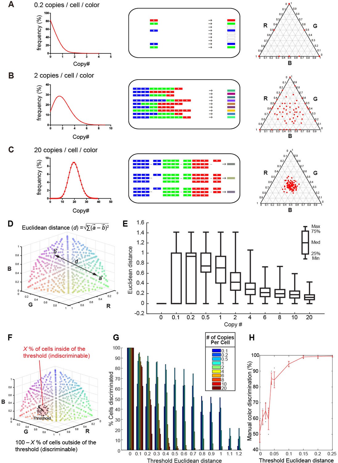
Tetbow strategy.
Stochastic representation of the vector-mediated multicolor labeling strategy. Here we assume that the copy numbers of introduced vectors follow a Poisson distribution. In a plasmid or virus-mediated gene transfer method, we do not need to use the Cre-loxP system. Rather, it is important to limit the number of genes introduced into each cell. For example, in theory, an average of 2 copies/cell/color can result in the stochastic expression of three different genes (B). If we introduce a copy number that is too small (e.g. an average of 0.2 copies/cell; A), only one of the three genes will be expressed in most cells. If too many genes are introduced in each cell (e.g. an average of 20 copies/cell; C), color variations will be reduced because many of the neurons will express a similar number of XFP genes. The use of the Cre-loxP system alone cannot solve this problem. Simulations of the expected color variations that are based on the various Poisson distributions (middle) are shown as ternary plots (100 plots/condition, right panel). The numerical data are presented in Figure 1—source data 1. Note that many of the plots are overlapping at the edge of the triangle in (A). Three different XFPs are shown in red (R), green (G), and blue (B). (D) The difference between two colors represented as Euclidean distance in 3D color space. For example, a difference between colors a and b is represented as the distance, d. (E) Box plots of Euclidean distances in all pairs of plots in 3D space in relation to copy number. The horizontal lines within each box represents the median, the box represents the interquartile range, and the whiskers show the minimum and maximum values. (F) A cartoon illustrating the cells inside (X%) and outside the threshold Euclidean distance. The cells outside (100 – X %) are considered to be discernable. (G) The percentage of discernable cells for each threshold d and each copy number. Simulation data used for (E) and (G) are provided in Figure 1—source data 1. (H) The color discrimination abilities of experienced researchers. Tests are explained in Figure 1—figure supplement 1. Mean ± SD are indicated in red. When threshold d is 0.1, the score was 94.5 ± 1.73% (mean ± SD). Score data are in Figure 1—source data 2.
-
Figure 1—source data 1
Simulation data used for Figure 1E, G.
- https://doi.org/10.7554/eLife.40350.005
-
Figure 1—source data 2
Color discrimination scores in Figure 1H.
- https://doi.org/10.7554/eLife.40350.006
Figure 1—figure supplement 1
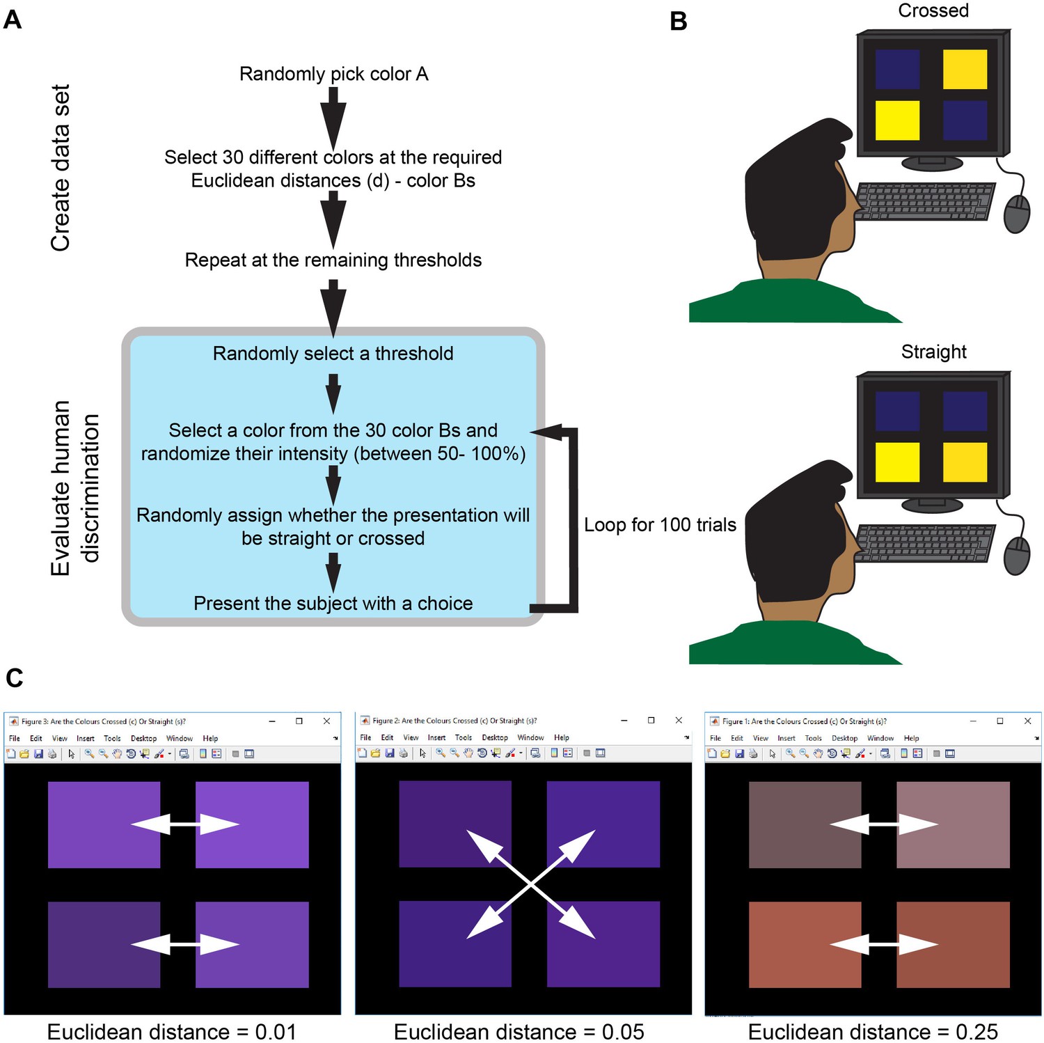
Explanation of human color discrimination tests.
(a) a flowchart describing the generation of the color sets and the user choices. The euclidean distances chosen as threshold values were 0, 0.01, 0.02, 0.03, 0.04, 0.05, 0.1, 0.15, 0.2, and 0.25. To prevent color intensity influencing decisions, the intensity was randomized in the 50–100% range for each trial. (b) a schematic showing either the ‘crossed’ (top) or ‘straight’ (bottom) decisions for the ‘same’ sets of colors that the user has to make. (c) examples showing the choices at various thresholds. White arrows display the correct decisions.
Figure 2 with 2 supplements
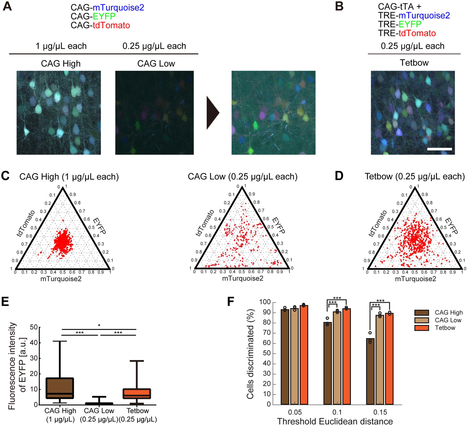
Bright multicolor labeling can be produced by using fewer copy numbers of plasmids with a stronger promoter.
(A) L2/3 neurons labeled with CAG-Turquoise2, EYFP, and tdTomato (1 or 0.25 μg/μL each). When each plasmid was introduced at 0.25 μg/μL, the color variation was increased, but the fluorescence levels were reduced. Enhanced images are shown on the right. (B) CAG-tTA, TRE- Turquoise2, EYFP, and tdTomato were introduced at 0.25 μg/μL each (Tetbow construct; see Figure 2—figure supplement 1). In utero electroporation was performed at E15 and the mice were analyzed at P21. Experiments were performed in parallel, and image acquisition conditions were the same for (A) and (B). Scale bars represent 50 μm. (C, D) Color variations made by three CAG vectors (C) vs. Tetbow vectors (D) are shown in ternary plots. Fluorescence intensities were vector normalized and the fluorescence intensity ratios were compared. Fluorescence intensities at neuronal somata were used for the quantitative comparison. Note that the color variations are small with high-copy CAG vectors, whereas color variations are high with the Tetbow vectors (n = 249–728 cells per group from three sets of experiments for each of the samples). Fluorescence intensity data used for (C), (D), and (F) are provided in Figure 2—source data 1. (E) Boxplot of median EYFP fluorescence intensities (normalized to the median of CAG (0.25 µg/µl). A D’Agostino and Pearson Normality Test showed that the data were not normally distributed (p<0.0001). EYFP signals in (A) and (B) were compared. The horizontal line in each box represents the median location, the box represents the interquartile range, and the whiskers show the minimum and maximum values. p*<0.05, p***<0.001 (Kruskal-Wallis with Dunn’s post hoc test, n = 104–276 per sample). The data are from one set of experiments performed in parallel. We analyzed three independent sets of experiments and obtained similar results. The fluorescence intensity data used for (E) are in Figure 2—source data 2. (F) Percentage of discernable cells in the condition of each threshold d and each copy number. p***<0.001 (two-way ANOVA with Tukey-Kramer post hoc test, n = 249–728 per sample).
-
Figure 2—source data 1
- https://doi.org/10.7554/eLife.40350.010
-
Figure 2—source data 2
Fluorescence intensity data used for Figure 2E.
- https://doi.org/10.7554/eLife.40350.011
Figure 2—figure supplement 1
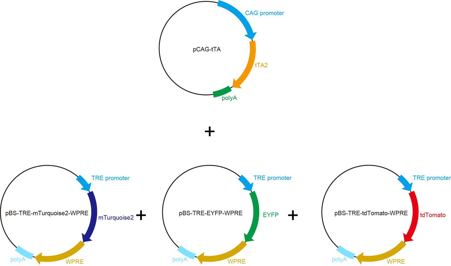
Tetbow constructs.
Plasmid maps for CAG-tTA, TRE-mTurquoise2/EYFP/tdTomato. To ensure adequate plasmid yield in Escherichia coli, the TRE expression cassette was transferred to a high-copy plasmid, pBluescriptII (SK+). To enhance the stability of mRNA, a WPRE sequence is added to the 3’’ UTR. We used cytosolic XFPs, because cytosolic XFPs are much brighter than membrane localized XFPs (data not shown).
Figure 2—figure supplement 2
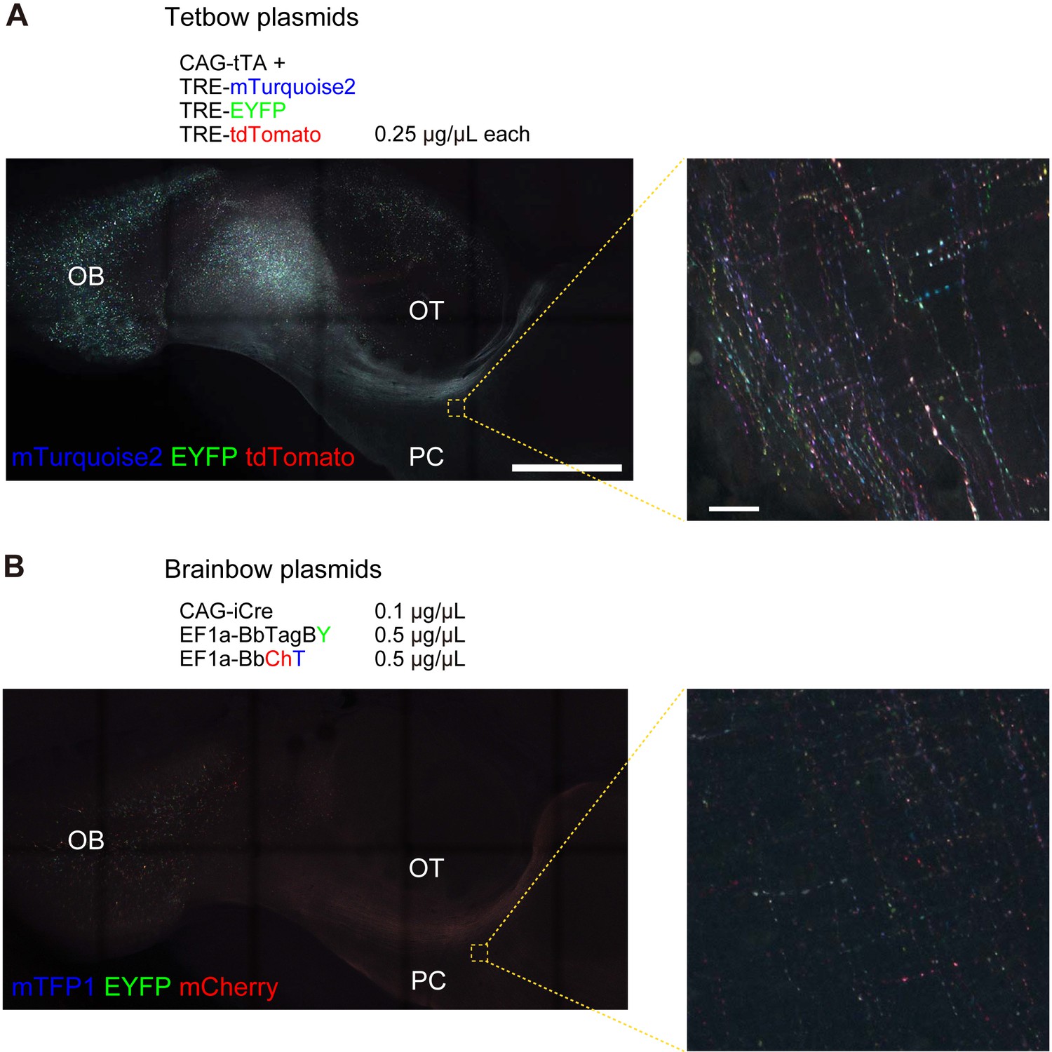
Comparison with Brainbow.
In utero electroporation was used to label M/T cells at E12 and mice were analyzed at P8. Whole brains were cleared with SeeDB2G and imaged with confocal microscopy. Low and high magnification images in axons of M/T cells are shown. High magnification images show the axon collaterals in the piriform cortex. (A) Tetbow constructs were introduced. Maximal intensity projection images of confocal images are shown (left: 1330.11 μm thick, right: 23.97 μm thick). (B) CAG-iCre (0.1 μg/μL), EF1a-BbTagBY (0.5 μg/μL), and EF1a-BbChT (0.5 μg/μL) were introduced. In utero electroporation was performed at E15 and mice were analyzed at P21. Experiments were performed in parallel, and image acquisition conditions were the same in (A) and (B). Note, however, that the Brainbow constructs use an EF1a promoter and membrane-bound XFPs, whereas Tetbow uses a TRE promoter and cytosolic XFPs. We also tested the CAG-Brainbow3.0 in the cerebral cortex, but labeling signals were much lower than Tetbow (data not shown). Scale bars are 1 mm (left) and 20 μm (right). Three samples were imaged in the same condition. A representative sample is shown for (A). The brightest sample is shown in (B), as we could not find clear signals at axons in the two remaining samples after clearing. OB, olfactory bulb; OT, olfactory tubercle, PC, piriform cortex.
Figure 3 with 1 supplement
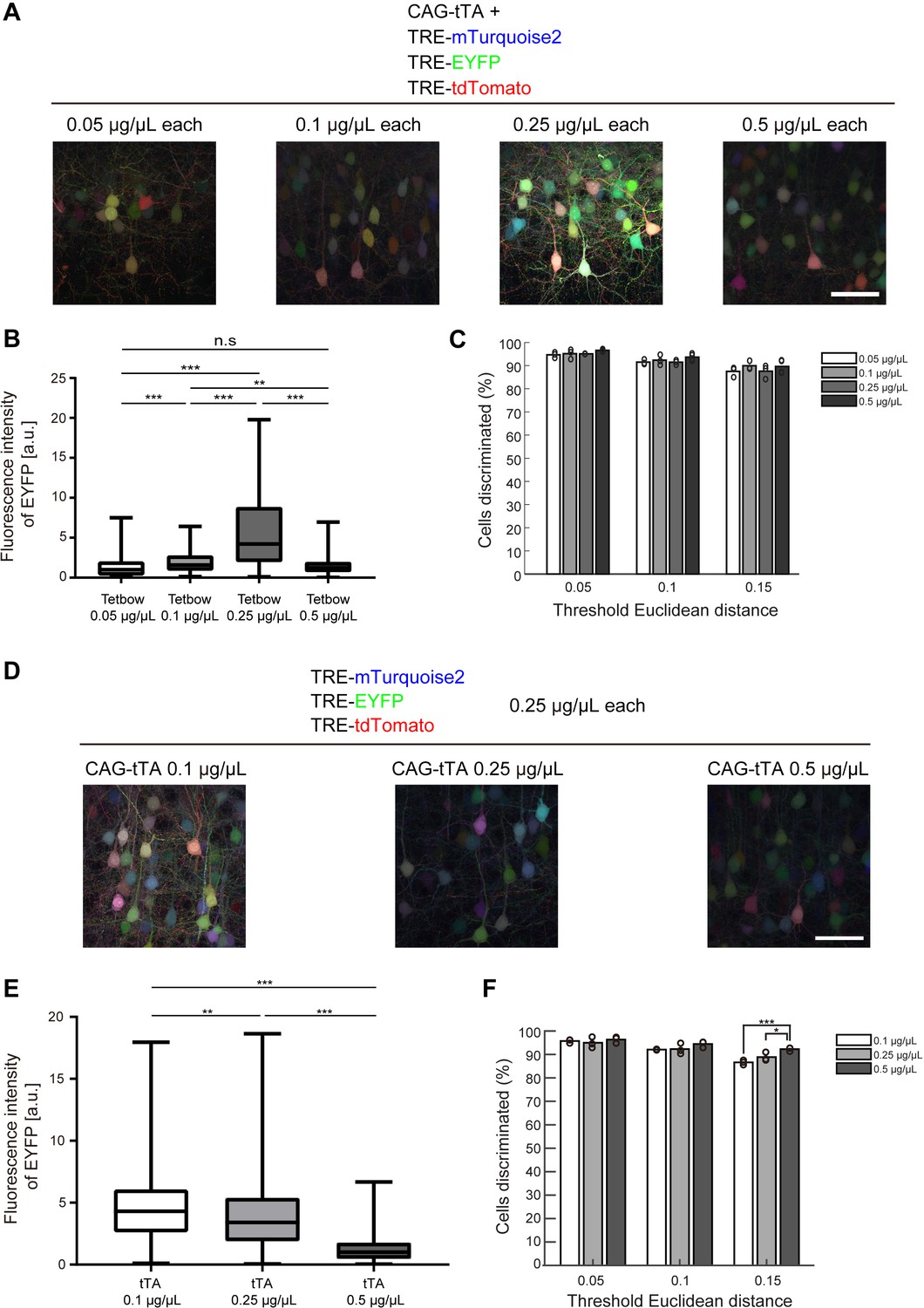
Optimization of Tetbow plasmid concentrations for in utero electroporation.
(A–C) Plasmid concentrations for the four Tetbow vectors (CAG-tTA and three TRE-XFP vectors) were tested at 0.05, 0.1, 0.25, and 0.5 μg/μL. (B) Boxplot of median EYFP fluorescence intensities (normalized to the median of Tetbow (0.05 µg/µl)). A D’Agostino and Pearson normality test showed that the data were not normally distributed (p<0.0001). The horizontal bar within each box represents the median fluorescence intensity, the box represents the interquartile range, and the whiskers show the minimum and maximum values. p**<0.01, p***<0.001 (Kruskal Wallis with Dunn’s post hoc test, n = 273–524 per sample). (C) Percentage of discernable cells for each of the threshold d and dilution conditions. There was no significant difference between each d condition (two-way ANOVA with Tukey-Kramer post hoc test) (n = 273–524 per sample). The fluorescence intensity data used for (B) and (C) are available in Figure 3—source data 1. (D–F) L2/3 neurons labeled with Tetbow. Only tTA concentrations were changed (0.1, 0.25, or 0.5 μg/μL). Decrease in tTA concentrations enhanced signal intensities. (E) Boxplot of median EYFP fluorescence intensities (normalized to the median of Tetbow (tTA: 0.5 µg/µl)). A D’Agostino and Pearson normality test showed that the data were not normally distributed (p<0.0001). The horizontal bar within each box represents the median location, the box represents the interquartile range, and the whiskers show the minimum and maximum values. p**<0.01, p***<0.001 (Kruskal Wallis with Dunn’s post hoc test, n = 356–414 per sample). (F) Percentage of discernable cells for each threshold d and each dilution condition. p*<0.05, p***<0.001 (two-way ANOVA with Tukey-Kramer post hoc test, n = 356–414 per sample). The fluorescence intensity data used for (E) and (F) are available in Figure 3—source data 2.
-
Figure 3—source data 1
Source data for Figure 3B,C.
- https://doi.org/10.7554/eLife.40350.014
-
Figure 3—source data 2
Source data for Figure 3E,F.
- https://doi.org/10.7554/eLife.40350.015
Figure 3—figure supplement 1
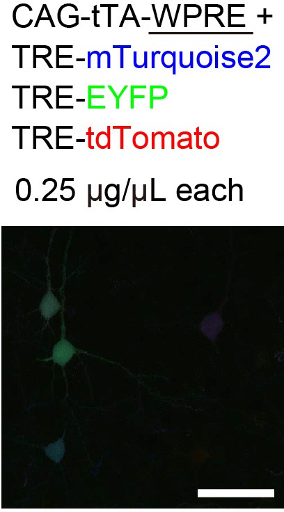
Tetbow optimization.
We tried to enhance the expression levels of XFPs by adding WPRE to the 3’′-UTR of the tTA gene, but the expression levels of XFPs were decreased with WPRE. The imaging conditions were the same as for Figure 2.
Figure 4 with 1 supplement
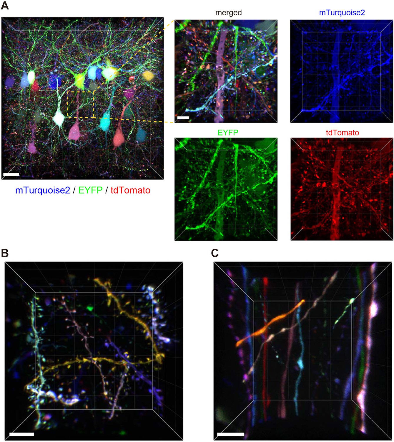
Tetbow labeling is bright enough for high-resolution imaging of synaptic structures.
Volume rendering of Layer 2/3 cortical pyramidal neurons labeled with Tetbow (P70). In utero electroporation was used to label L2/3 neurons at E15. Brain slices were cleared with SeeDB2G and imaged with confocal microscopy. Different neurons were brightly labeled with different colors. Representative images are shown from four independent experiments. (A) Low- and high-magnification images in Layer 2/3 (45.16 μm thick). The four panels on the right indicate each of the three single channel fluorescence images. See also Video 1. (B) Dendrites and dendritic spines were brightly labeled with various colors with Tetbow. A volume-rendered image (18.65 μm thick) is shown. See also Video 2. (C) Axons and axonal boutons were clearly visualized with Tetbow. A volume rendered image (23.01 μm thick) is shown. Note that the synaptic-scale structures were clearly visualized with the native fluorescence of XFPs, without antibody staining. Scale bars are 20 μm (A, left) and 5 μm (A, right and B, C).
Figure 4—figure supplement 1
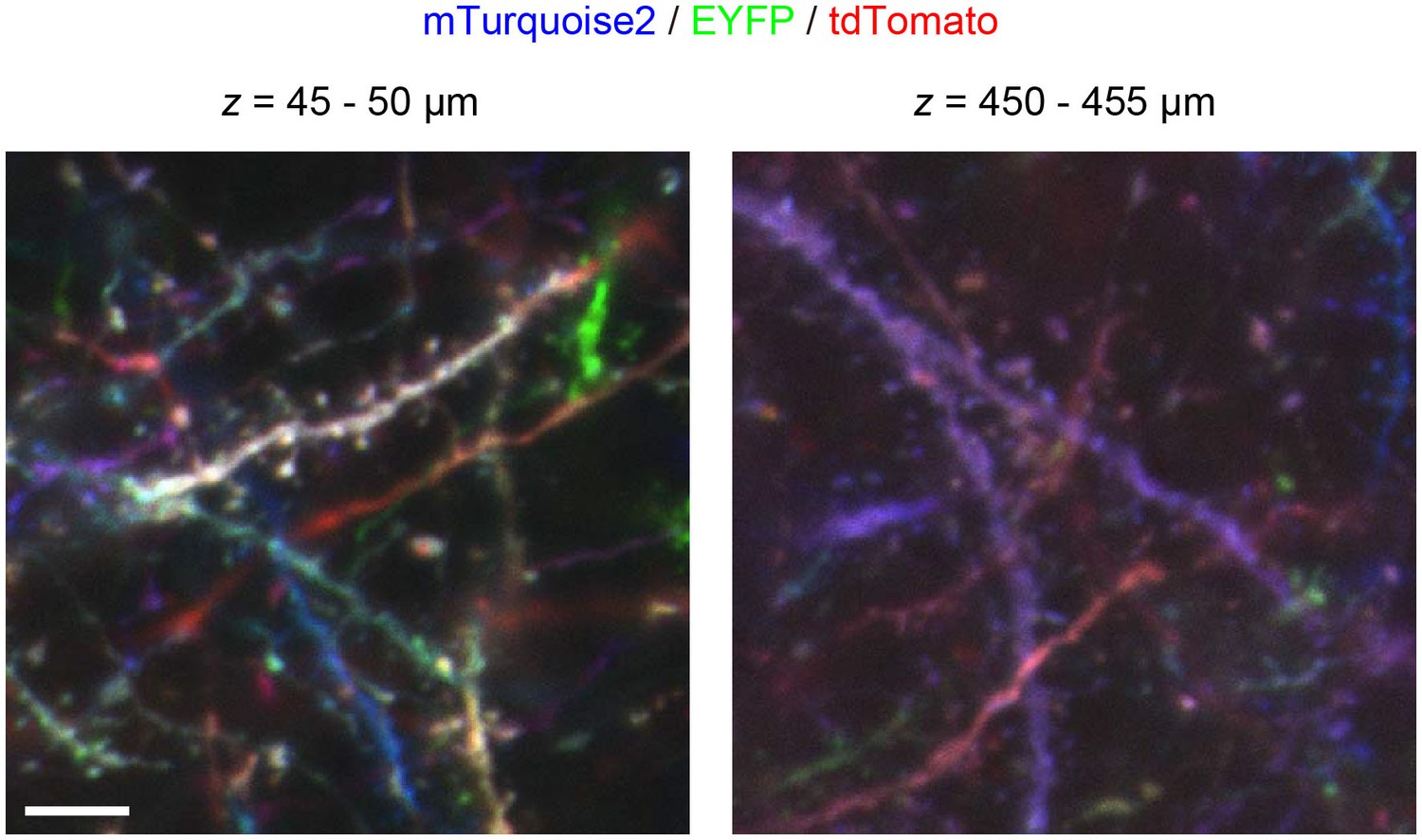
Tetbow labeling is bright enough in thick brain slices.
Shallow and deep images of L2/3 cortical pyramidal neurons labeled with Tetbow in a thick brain slice (1 mm). In utero electroporation was used to label L2/3 neurons at E15. Brain slices were cleared with SeeDB2G and imaged with confocal microscopy. Maximal intensity projection images of confocal images are shown (4.96 μm thick). Dendritic spines were visualized in the deep section of thick slices. Scale bars are 5 μm.
Figure 5
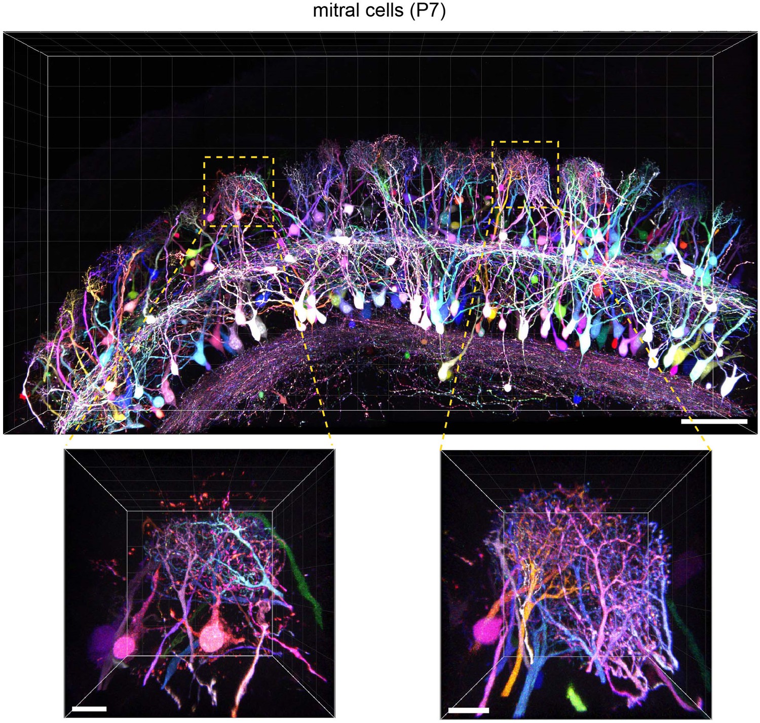
Tetbow labeling in the olfactory bulb.
M/T cells in the olfactory bulb (P7) were labeled with Tetbow. A volume-rendered image is shown (84.07 μm thick). Each mitral cell was labeled with unique colors facilitating the identification of individual neurons at high resolution. Note that dendritic tufts from different neurons are clearly distinguishable with different colors in the high-magnification image (bottom). Representative data from one out of three independent experiments are shown here. See also Video 3. Scale bars are 100 μm (top) and 20 μm (bottom). Fluorescence signals at M/T cell somata are intentionally saturated in this image so that the fine details of dendrites are better visualized.
Figure 6 with 2 supplements
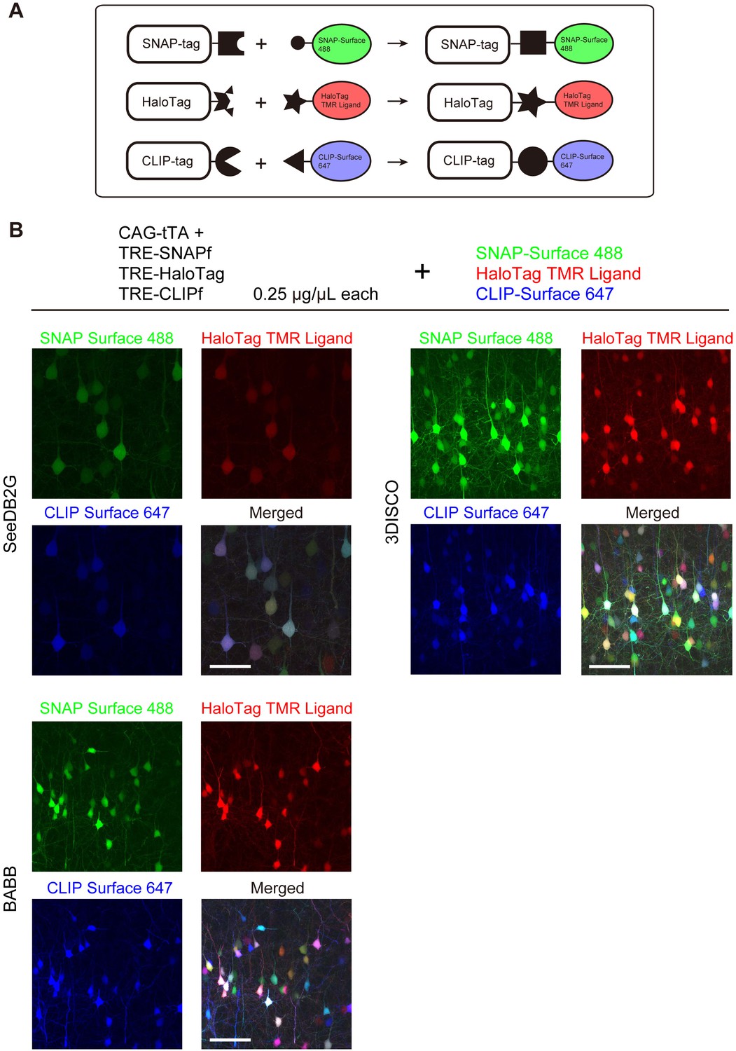
Tetbow labeling with chemical tags.
(A) Tetbow labeling with chemical tags. We used SNAP, CLIP, and Halo tags for Tetbow labeling. These chemical tags form covalent bonds with their substrates, which contain chemical fluorophores. These chemical labels are stable even under harsh clearing conditions. See Figure 6—figure supplement 1 for plasmid construction. (B) L2/3 neurons labeled with SNAP, Halo, and CLIP tags were visualized with SNAP-Surface 488, HaloTag TMR Ligand, and CLIP-Surface 647 (P21), respectively. Brain tissue was cleared with SeeDB2G, BABB, or 3DISCO. Note that a fluorescent protein, mTurquoise2, was largely quenched by BABB and 3DISCO whereas chemical tags with synthetic dyes remained stable. Scale bars are 50 μm. Data for each condition were obtained from sections from the same animal. This process was replicated for three animals.
Figure 6—figure supplement 1
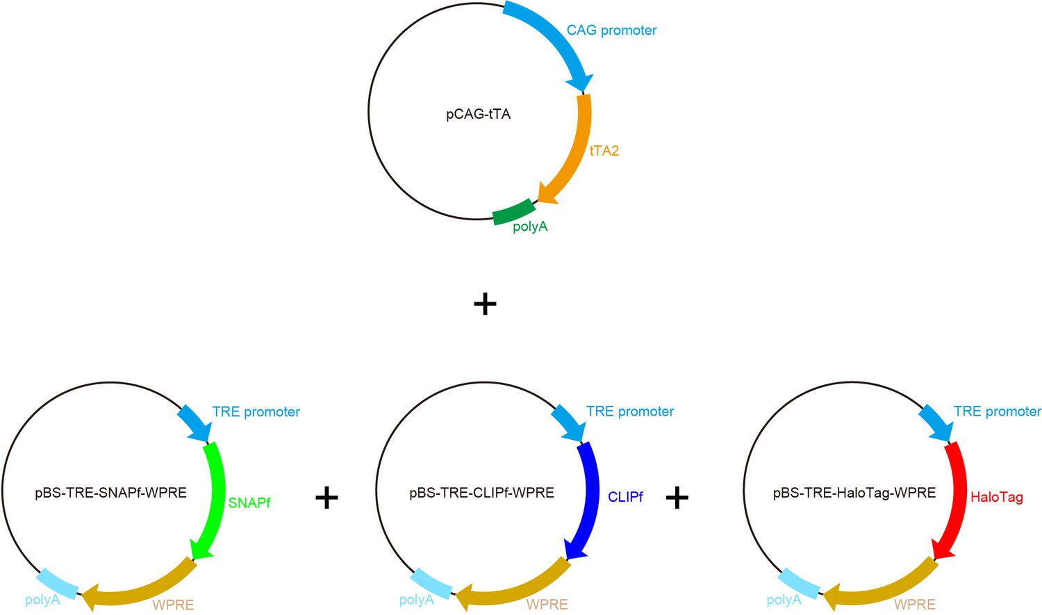
Plasmid maps for chemical-tag Tetbow.
Plasmid maps for a chemical-tag Tetbow. Chemical-tag expression cassettes are basically the same as those for XFPs.
Figure 6—figure supplement 2

Efficient labeling of thick brain slices with chemical tags.
L2/3 neurons labeled with SNAP, Halo, and CLIP tags were visualized with SNAP-Surface 488, HaloTag TMR Ligand, and CLIP-Surface 647, respectively. Chemical tag genes were introduced by in utero electroporation at E15. A 1-mm-thick brain slice (P21) was cleared with SeeDB2G. Scale bars are 50 μm.
Figure 7 with 2 supplements

Tetbow labeling with AAVs.
(A) Layer five pyramidal neurons in the cerebral cortex labeled with Tetbow AAVs. Tetbow AAVs (serotype AAV2/1) were injected at P56 and analyzed two weeks later. Brain slices were cleared with SeeDB2G. The images display the native fluorescence of XFPs under SeeDB2G clearing. Low- and high-magnification images (89 μm thick, volume rendering) are shown. Scale bars are 100 μm on the left, and 10 μm on the right. (B) The optimization of virus titer conditions. Various titers of TRE-mTurquoise2, TRE-EYFP and TRE-tdTomato (1 × 10¹⁰, 3 × 10¹⁰, 1 × 10¹¹ gc/mL) were injected at P56 and analyzed two weeks later. The tTA titer was 4 × 10⁸ gc/mL throughout. (C) Boxplots of EYFP fluorescence intensities at the cell bodies (normalized to the median of 1 × 10¹⁰ gc/mL). A D’Agostino and Pearson normality test showed that the data were not normally distributed (p<0.0001). The horizontal line within each box represents the median location, the box represents the interquartile range, and the whiskers represent the minimum and maximum values. p*<0.05, p***<0.001 (Kruskal-Wallis with Dunn’s post hoc test, n = 163–220 per sample). (D) The percentage of discernable cells for each threshold d and each titer condition. p*<0.05, p**<0.01, p***<0.001 (two-way ANOVA with Tukey-Kramer post hoc test, n = 163–220 per sample). Fluorescence intensity data used for (B) to (D) are available in Figure 7—source data 1.
-
Figure 7—source data 1
Fluorescence intensity data used for Figure 7B-D.
- https://doi.org/10.7554/eLife.40350.028
Figure 7—figure supplement 1
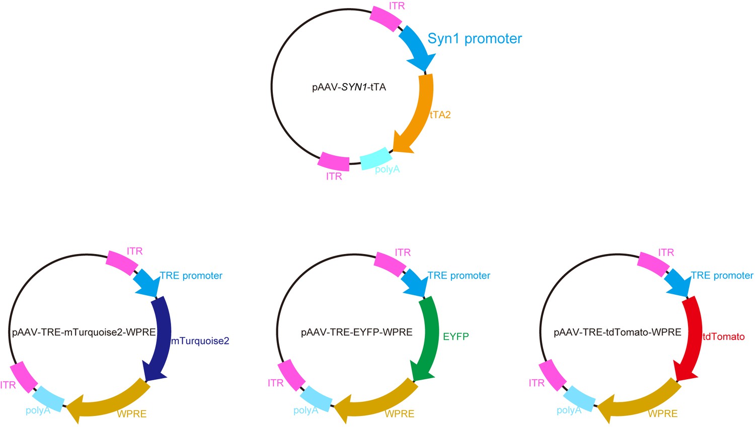
AAV vector maps.
Plasmid maps for the pAAV vectors used in this study. TRE-XFP expression cassettes are basically the same as in in utero electroporation. The tTA gene was expressed under the SYN1 promoter to ensure neuronal expression.
Figure 7—figure supplement 2
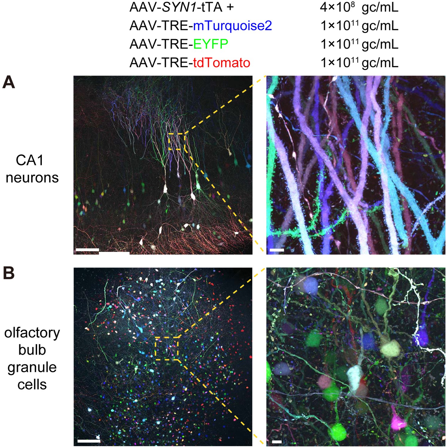
Various brain areas labeled with Tetbow AAVs.
(A) CA1 neurons in the hippocampus labeled with Tetbow AAVs. See also Video 4. (B) Granule cells in the olfactory bulb labeled with Tetbow AAVs. Tetbow AAVs were injected at P56 and analyzed two weeks later. Brain slices were cleared with SeeDB2G. Note that fine dendritic spines are clearly visualized with different color hues. Images are native fluorescence of XFPs under SeeDB2G clearing. Maximal intensity projection images of confocal images are shown (234.62 μm thick for (A), and 272 μm thick for (B)). Scale bars are 100 μm in the panels on the left, and 5 μm in those on the right. Fluorescence intensity data used for (B)-(D) are available in Figure 7—source data 1.
Figure 8 with 2 supplements
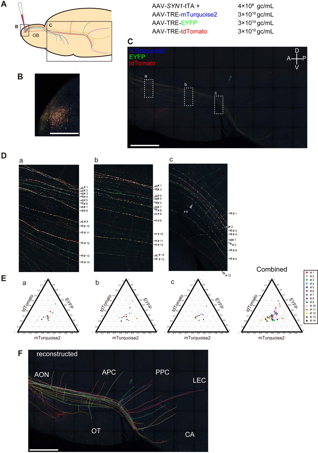
Long-range tracing of M/T cell axons with Tetbow AAVs.
(A) M/T cells in the olfactory bulb were labeled with Tetbow AAVs. The Tetbow AAV cocktail (138 nL) was injected into a single location on the dorsal surface of the right olfactory bulb using a glass capillary. The virus was injected at P60 and mice were analyzed four weeks later. AAV titers were 4 × 10⁸ gc/mL for AAV2/1-SYN1-tTA2 and 3 × 10¹⁰ gc/mL each for AAV2/1-TRE-mTurquoise2-WPRE, AAV2/1-TRE-EYFP-WPRE, and AAV2/1-TRE-tdTomato-WPRE. (B) In the olfactory bulb, M/T cells and various types of interneurons were densely labeled with Tetbow. (C) In the olfactory cortex, only M/T cell axons were labeled with Tetbow AAVs. The ventral-lateral part of the brain was flattened to 700 μm thickness. After fixation and clearing, confocal images were taken with 20x objective lenses. The labeling density was lower in the olfactory cortex, so we could easily trace individual M/T cell axons. M/T cell axons were found in the all areas of the olfactory cortex, including anterior olfactory nucleus (AON), olfactory tubercle (OT), piriform cortex (anterior (APC) and posterior (PPC)), cortical amygdala (CA), and lateral entorhinal cortex (LEC). Maximal intensity projection images of confocal images are shown (379.89 μm). See also Video 5. (D) High-magnification versions of the images shown in (C). All of the axons that were found in both area (a) and (b) and that could be traced for >1,000 μm were analyzed (14 axons). (E) Ternary plots of color codes in the axons highlighted in (C). Average color codes in each area (a–c) are shown. The color consistency is shown on the right. The color code was largely consistent across the areas except for a few axons (#6, #11 or #12). The copy number may not be optimum in this sample, as the plots are not found in the periphery of the ternary plots. The fluorescence intensity data used for (E) are available in Figure 8—source data 1. (F) Tracing and reconstruction of M/T cell axons. We terminated tracing when the labeled axons were interrupted by unlabeled gaps. Thus, our conservative tracing is most probably showing an underestimate of the entire wiring diagram. All of the axons that could be successfully traced for >1,000 μm are shown. The maximum length of the traced axon was 6852.63 μm. A z-stacked image of the reconstruction is shown. Tracings of individual M/T cells are shown in Figure 8—figure supplement 2. See also Video 6. Scale bars are 1 mm.
-
Figure 8—source data 1
Fluorescence intensity data used for Figure 8E.
- https://doi.org/10.7554/eLife.40350.034
-
Figure 8—source data 2
Axon length data used for Figure 8—figure supplement 1D.
- https://doi.org/10.7554/eLife.40350.033
Figure 8—figure supplement 1
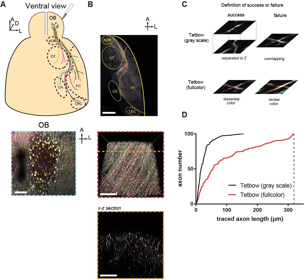
Comparison of the tracing performances of single-color and Tetbow labeling using dense axon labeling.
(A) Olfactory bulb neurons were densely labeled with Tetbow AAVs. The majority of M/T cells in the dorsal olfactory bulb were labeled. AON, anterior olfactory nucleus; CA, cortical amygdala; LEC, lateral entorhinal cortex; OB, olfactory bulb; OT, olfactory tubercle; PC, piriform cortex. (B) M/T cell axons were densely labeled in the lateral olfactory tract. An enlarged image of the red boxed area is shown below. A z-stack image of and an image of the x-z section along the orange line are shown. Using this sample, we compared the tracing performance of single-color vs. Tetbow labeling. (C) The definition of successful tracing. In the gray-scale image data, we judged that two axons were successfully dissected when they crossed-over at different z positions (success). We judged that axon tracing failed when the two axons crossed on the same z plane (failure). In Tetbow tracing (full color), we judged that two axons were successfully dissected when the color hues for the two axons were visually discernable (success). We judged that the tracing failed when the two axons crossed on the same z plane and the two colors were visually too alike to discriminate (failure). According to Figure 1H, an experimenter can discriminate between two different colors separated by Euclidean distance 0.1 at >90% accuracy. We did not consider the direction of the crossing axons when we made a decision of success vs. failure. (D) Cumulative plots showing successfully traced axon length. The maximum length of traced axons in the gray-scale image data was 155.229 μm. The maximum length of traced axons in Tetbow (full color) was 318.953 μm. Eight axons out of 100 were fully traced Tetbow (full color), whereas no axons could be fully traced in the gray-scale image. Thus, Tetbow labeling much improves the tracing performance for densely labeled axons. Scale bars are 100 μm (A), 1 mm (B, top), and 50 μm (B, middle and bottom).
Figure 8—figure supplement 2
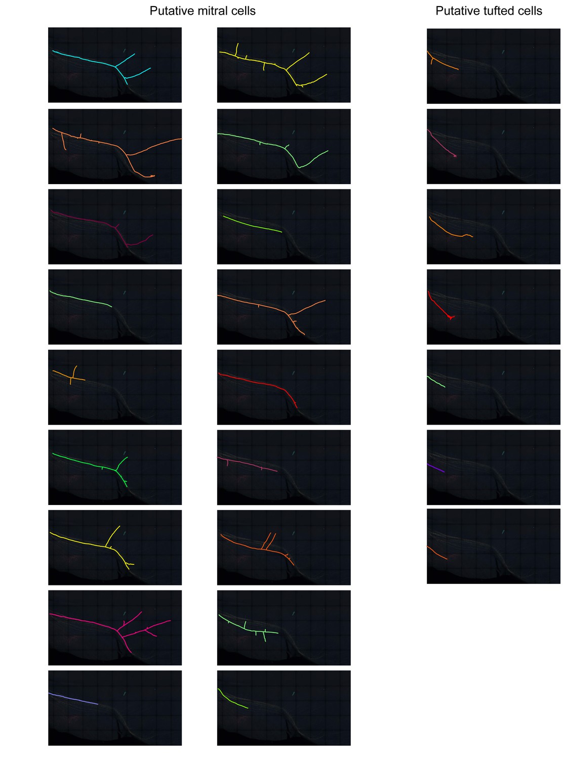
Traced M/T cell axons in Figure 8F shown separately.
Putative mitral cell axons travel along the distal part of the lateral olfactory tract and send collaterals to the piriform cortex. Putative tufted cell axons terminate in the olfactory tubercle.
Videos
Video 1
Layer 2/3 cortical pyramidal neurons labeled with Tetbow.
Tetbow plasmids were introduced at E15 and the cerebral cortex was analyzed at P70. See legends to Figure 4A.
Video 2
High-magnification images of dendrites in Layer 2/3 cortical pyramidal neurons labeled with Tetbow.
Tetbow plasmids were introduced at E15 and the cerebral cortex was analyzed at P70. See legends to Figure 4B.
Video 3
Mitral cells of the olfactory bulb labeled with Tetbow.
Tetbow plasmids were introduced at E12 and the olfactory bulb samples were analyzed at P7. See legends to Figure 5.
Video 4
CA1 pyramidal neurons in the hippocampus labeled with Tetbow AAVs.
Tetbow AAVs were injected to the hippocampus at P56 and analyzed after two weeks. See legends to Figure 7—figure supplement 2.
Video 5
M/T cell axons sparsely labeled with Tetbow AAVs.
Tetbow AAVs were injected to the olfactory bulb at P60 and analyzed after four weeks. Volume-rendering images of the olfactory cortex are shown. See legends to Figure 8.
Video 6
Reconstruction of M/T cells axons.
Traced M/T cell axons are separately shown. See legends to Figure 8 and Figure 8—figure supplement 1.
Tables
Key resources table
| Reagent type (species) or resource | Designation | Source or reference | Identifiers | Additional information | ||
|---|---|---|---|---|---|---|
| Gene (Mus musculus) | C57BL/6N | Japan SLC | RRID: MGI:5658686 | |||
| Gene (Mus musculus) | ICR | Japan SLC | RRID: MGI:5652524 | |||
| Cell line (Homo sapiens) | AAVpro 293 T Cell Line | Clontech | cat# 632273 | |||
| Recombinant DNA reagent | pTRE-Tight | Clontech | cat# 631059 | |||
| Recombinant DNA reagent | pCAG-CreERT2 | PMID: 17209010 (Matsuda and Cepko, 2007) | Addgene# 14797 | |||
| Recombinant DNA reagent | pmTurquoise2-N1 | PMID: 22434194 (Goedhart et al., 2012;Matsuda and Cepko, 2007) | Addgene# 60561 | |||
| Recombinant DNA reagent | pBluescript II SK(+) phagemid | Agilent Technologies | cat# 212205 | |||
| Recombinant DNA reagent | paavCAG-pre- mGRASP-mCerulean | PMID: 22138823 (Kim et al., 2011) | Addgene# 34910 | |||
| Recombinant DNA reagent | pSNAPf | New England Biolabs | cat# N9183S | |||
| Recombinant DNA reagent | pCLIPf | New England Biolabs | cat# N9215S | |||
| Recombinant DNA reagent | pFC14K HaloTag CMV Flexi Vector | Promega | cat# G3780 | |||
| Recombinant DNA reagent | pCAG-mTurquoise2 | This paper | N/A | |||
| Recombinant DNA reagent | pCAG-EYFP | This paper | N/A | |||
| Recombinant DNA reagent | pCAG-tdTomato | This paper | N/A | |||
| Recombinant DNA reagent | pCAG-tTA | This paper | Addgene# 104102 | |||
| Recombinant DNA reagent | pBS-TRE -mTurquoise2-WPRE | This paper | Addgene# 104103 | |||
| Recombinant DNA reagent | pBS-TRE-EYFP-WPRE | This paper | Addgene# 104104 | |||
| Recombinant DNA reagent | pBS-TRE-td Tomato-WPRE | This paper | Addgene# 104105 | |||
| Recombinant DNA reagent | pBS-TRE-SNAPf-WPRE | This paper | Addgene# 104106 | |||
| Recombinant DNA reagent | pBS-TRE-CLIPf-WPRE | This paper | Addgene# 104107 | |||
| Recombinant DNA reagent | pBS-TRE-HaloTag-WPRE | This paper | Addgene# 104108 | |||
| Recombinant DNA reagent | AAV2-miniSOG -VAMP2-tTA-mCherry | PMID: 23889931 (Lin et al., 2013) | Addgene# 50970 | |||
| Recombinant DNA reagent | pAAV-SYN1-tTA | This paper | Addgene# 104109 | |||
| Recombinant DNA reagent | pAAV-TRE -mTurquoise2-WPRE | This paper | Addgene# 104110 | |||
| Recombinant DNA reagent | pAAV-TRE -EYFP-WPRE | This paper | Addgene# 104111 | |||
| Recombinant DNA reagent | pAAV-TRE -tdTomato-WPRE | This paper | Addgene# 104112 | |||
| Recombinant DNA reagent | pCAG-iCre | PMID: 26972009 (Ke et al., 2016) | N/A | |||
| Recombinant DNA reagent | AAV-EF1a-BbTagBY | PMID: 23817127 (Cai et al., 2013) | Addgene# 45185 | |||
| Recombinant DNA reagent | AAV-EF1a-BbChT | PMID: 23817127 (Cai et al., 2013) | Addgene# 45186 | |||
| Commercial assay or kit | AAVpro Helper Free System | Takara | cat# 6673 | |||
| Commercial assay or kit | AAVpro Purification Kit (All Serotypes) | Takara | cat# 6666 | |||
| Commercial assay or kit | AAVpro Titration Kit (for real-time PCR) | Takara | cat# 6233 | |||
| Chemical compound, drug | SNAP-Surface 488 | New England Biolabs | cat# S9124S | |||
| Chemical compound, drug | CLIP-Surface 647 | New England Biolabs | cat# S9234S | |||
| Chemical compound, drug | HaloTag TMR Ligand | Promega | cat# G8252 | |||
| Chemical compound, drug | Saponin | Nakalai-tesque | cat# 30502–42 | |||
| Chemical compound, drug | Omnipaque 350 | Daiichi-Sankyo | cat# 081–106974 | |||
| Chemical compound, drug | Urea | Wako | cat# 219–00175 | |||
| Chemical compound, drug | N,N,N',N'-Tetrakis (2-hydroxypropyl) ethylenediamine | TCI | cat# T0781 | |||
| Chemical compound, drug | Triton X-100 | Nakalai-tesque | cat# 12967–45 | |||
| Chemical compound, drug | Hexane | Nakalai-tesque | cat# 17922–65 | |||
| Chemical compound, drug | Benzyl alcohol | SIGMA | cat# 402834–100 ML | |||
| Chemical compound, drug | Benzyl benzoate | Wako | cat# 025–01336 | |||
| Chemical compound, drug | Tetrahydrofuran, super dehydrated, with stabilizer | Wako | cat# 207–17905 | |||
| Chemical compound, drug | Dibenzyl Ether | Wako | cat# 022–01466 | |||
| Software, algorithm | ImageJ | NIH | RRID: SCR_003070 | |||
| Software, algorithm | GraphPad Prism 7 | GraphPad Software | RRID: SCR_002798 | |||
| Software, algorithm | MATLAB | MathWorks | RRID: SCR_001622 | |||
| Software, algorithm | Leica Application Suite X | Leica Microsystems | RRID: SCR_013673 | |||
| Software, algorithm | Imaris | Bitplane AG | RRID: SCR_007370 | |||
| Software, algorithm | Neurolucida | MBF Bioscience | RRID: SCR_001775 | |||
| Software, algorithm | Adobe Photoshop | Adobe | RRID: SCR_014199 | |||
| Software, algorithm | Adobe Illustrator | Adobe | RRID: SCR_010279 | |||
| Other | Microslicer | Dosaka EM | PRO7N | |||
| Other | Electroporator | BEX | CUY21EX | |||
| Other | Forceps-type electrodes (5 mm diameter) | BEX | LF650P5 | |||
| Other | Forceps-type electrodes (3 mm diameter) | BEX | LF650P3 | |||
| Other | TCS SP8X | Leica Microsystems | TCS SP8X | |||
| Other | 10x dry lens | Leica Microsystems | HC PL APO 10x/0.40 CS | |||
| Other | 20x multi-immersion objective lens | Leica Microsystems | HC PL APO 20x /0.75 IMM CORR CS2 | |||
| Other | 40x oil-immersion objective lens | Leica Microsystems | HC PL APO 40x OIL CS2, | |||
| Other | 63x glycerol-immersion objective lens | Leica Microsystems | HC PL APO 63x GLYC CORR CS2 | |||
| Other | Raw image data | This paper | http://ssbd.qbic.riken.jp/set/20180901/ | |||
| Other | Neurolucida reconstruction data | This paper | http://ssbd.qbic.riken.jp/set/20180901/ | |||
| Other | MATLAB codes | This paper | https://github.com/mleiwe/TetbowCodes | |||
Additional files
-
Transparent reporting form
- https://doi.org/10.7554/eLife.40350.037
Download links
A two-part list of links to download the article, or parts of the article, in various formats.
Downloads (link to download the article as PDF)
Open citations (links to open the citations from this article in various online reference manager services)
Cite this article (links to download the citations from this article in formats compatible with various reference manager tools)
Bright multicolor labeling of neuronal circuits with fluorescent proteins and chemical tags
eLife 7:e40350.
https://doi.org/10.7554/eLife.40350


