Cellular cartography of the organ of Corti based on optical tissue clearing and machine learning
- The University of Tokyo, Japan
- Kyoto University, Japan
Figures
Figure 1 with 2 supplements
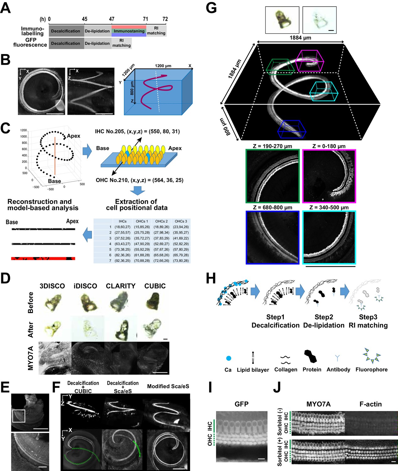
Optical tissue clearing and whole-mount immunolabeling of the organ of Corti.
(A) Time course and individual steps of tissue clearing with or without immunostaining. (B) Three-dimensional imaging of the organ of Corti within the temporal bone. Top view (left), lateral view (middle), and the schematic presentation of the organ of Corti with its axis parallel to the modiolus. The size of the organ of Corti is indicated in the X, Y, and Z coordinates. Scale bar, 500 μm. (C) Computational processes of linearization, cell detection, and modeling. (D) Side-by-side comparison of 3DISCO, iDISCO, CLARITY, and CUBIC. Transmitted light images of samples before and after clearing, together with MYO7A staining. Scale bar, 500 μm. (E) Manual dissection of the iDISCO-processed sample confirmed MYO7A staining in the sensory epithelium. Scale bars, 500 μm (upper image) and 100 μm (lower image). (F) Lateral and horizontal views of the reconstructed three-dimensional images of the organ of Corti stained with anti-MYO7A. CUBIC with decalcification and original ScaleS failed to detect the deepest part of the organ of Corti (green dotted lines). With modified ScaleS, the entire structure of the organ of Corti could be visualized. Scale bar, 500 μm. (G) Modified ScaleS sample of the organ of Corti stained with anti-MYO7A antibody, together with transmitted light images before (upper left) and after (upper right) treatment. Scale bar, 500 μm. (H) Three steps of the modified ScaleS protocol. The initial decalcification step is followed by a clearing step, which mainly removes lipids from the extracellular matrix. Finally, the RI of the sample is matched with mounting solution. (I) Preservation of GFP fluorescence after modified ScaleS treatment. Scale bar, 10 μm. (J) Preservation of rhodamine-phalloidin signal after modified ScaleS treatment, which includes sorbitol to stabilize cytoskeletal polymers. Scale bar, 10 μm. IHC, inner hair cell; OHC, outer hair cell; RI, refractive index.
-
Figure 1—source data 1
Source data for Figure 1B, E and Figure 1—figure supplement 2.
- https://doi.org/10.7554/eLife.40946.005
Figure 1—figure supplement 1
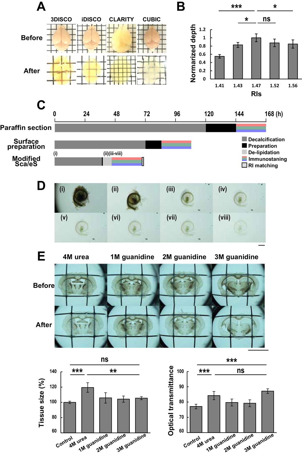
Protocol of modified Sca/eS.
(A) Comparison of optical transparency of mouse brain samples using 3DISCO, iDISCO, CLARITY and CUBIC. Scale, 3 mm. (B) Relationship between imaging depths and RIs using the decalcified cochlea as a sample. (n = 5 samples. Dunnet’s multiple comparison test, *p < 0.05; ***p < 0.001; ns; not significant, p > 0.05.) (C) Time course and individual steps of modified Sca/eS compared to the previous protocols of cochlear tissue preparations. (D) Macroscopic images of the cochlea through the steps of decalcification, clearing, and RI matching. Each image corresponds to the time points (i) to (viii) shown in (A). Scale bar, 1 mm. (E) Mouse brain sections with 100 μm thickness were treated with urea and guanidine solutions at varying concentrations. After tissue clearing, tissue volume expansion and optical transmittance were measured. Scale bar, 5 mm. (n = 5 samples for each condition. One-way ANOVA with Bonferroni’s post hoc test, *p < 0.05; ***p < 0.001; ns; not significant, p > 0.05.) RI, refractive index.
Figure 1—figure supplement 2

Application of modified ScaleS to other tissues.
(A) Tubular bone samples were treated with modified ScaleS and CB-perfusion. CB-perfusion was designed for whole-body imaging (see Appendix 1 for the detail). Transmitted light Images before and after clearing procedures were presented. The trabecular regions of the tubular bone (boxed regions of the low magnification images with transmitted light) stained with anti-vascular endothelial (VE)-cadherin were imaged through the surface of the compact bone. Boxed regions in fluorescence images were further enlarged for presentation of vasculature details. Scale bar, 5 mm (transmission images), 100 μm (fluorescence images). The graph shows the maximal depth at which the VE-cadherin signals could be detected from the surface. (n = 3 samples for each condition. Two-tailed unpaired t test, *p < 0.05.) (B) Application of modified ScaleS to multiple biological samples. To test the effectiveness of modified ScaleS for clearing the non-osseous tissue, multiple organs (brain, heart, stomach, lung, liver, kidney, intestine and spleen) were processed with modified ScaleS and CB-perfusion. Performance of CB-perfusion was better than modified ScaleS in stomach, lung, liver, kidney and spleen. This difference can be explained by better performance of CB-perfusion in elimination of blood cells by perfusion and effective delipidation and decolorization by aminoalcohol. Scale bar, 5 mm.
Figure 2 with 2 supplements
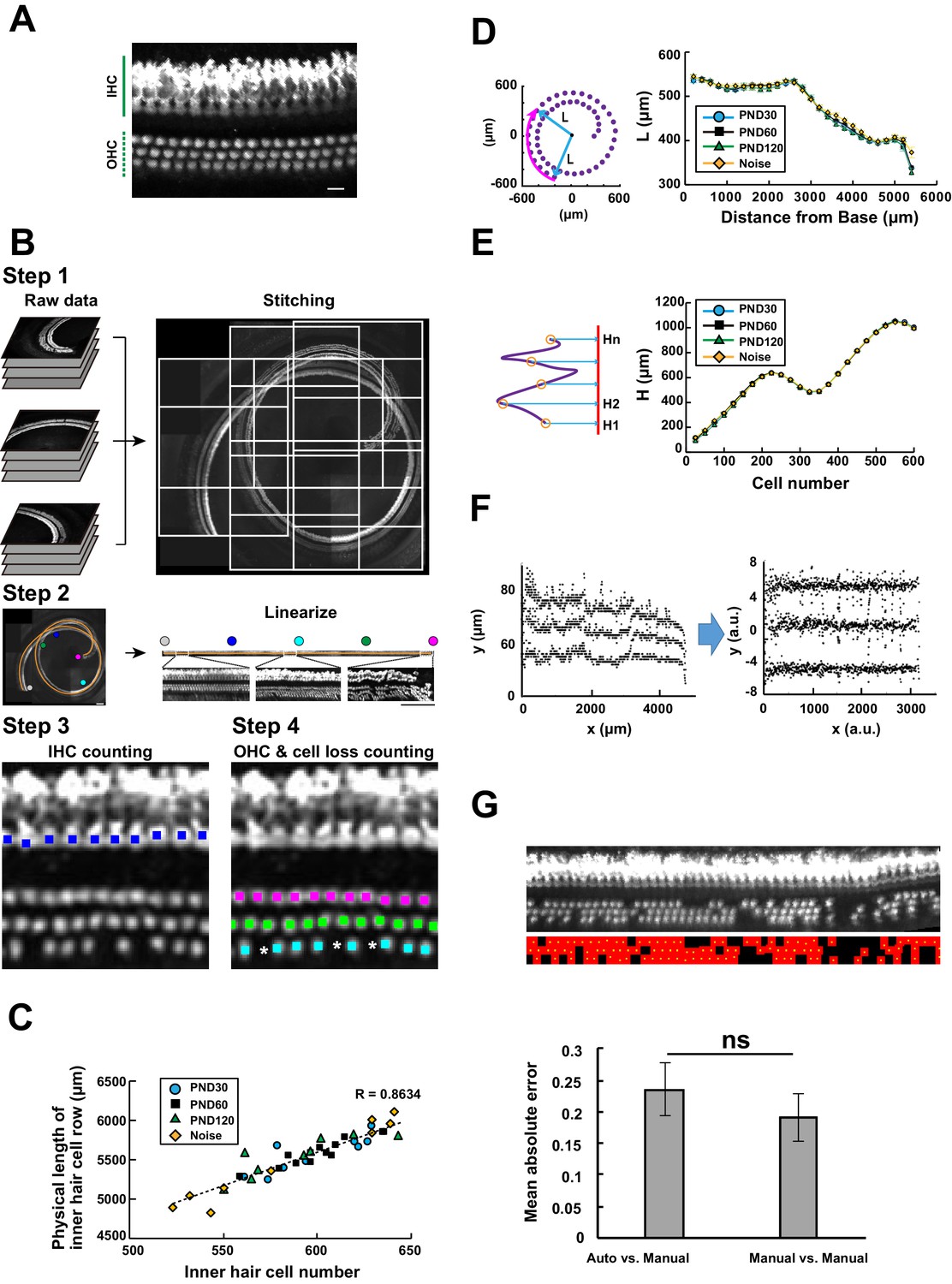
Computational analysis of hair cell distribution in the organ of Corti.
(A) Detection of single hair cells stained with anti-MYO7A. The border between hair cells can be clearly detected. Scale bar, 10 μm. (B) Sequential steps in reconstruction of the linearized voxel image of the organ of Corti. The linearized voxel image was generated using the row of IHCs as a structural reference of the longitudinal axis of the organ of Corti. Scale bar, 100 μm. (C) Plot of the total longitudinal length of the organ of Corti against the total number of IHCs. (D) Plot of radial distance of IHCs from the modiolus. (E) Plot of hair cell positions along the vertical axis of the organ of Corti. (F) Normalization of heterogeneity in hair cell positions. Before normalization, both x and y axes represent physical positions of OHCs. After normalization, the coordinates are arbitrary units and are equalized in x and y axes. (G) Transformation of the positions of hair cells to fit the standardized template. The template is a two-dimensional grid parallel to the surface of the sensory epithelium (upper image). This transformation is useful for estimation of lost hair cells based on the calculation of cell-free space. The accuracy of estimation by this method was comparable to the performance of manual estimation (lower plot). [n = 161 samples for each. Paired t-test; ns, not significant (p > 0.05).] IHC, inner hair cell; OHC, outer hair cell; PND, postnatal day; RI, refractive index.
-
Figure 2—source data 1
Source data for Figure 2D, E, G and Figure 2—figure supplement 1.
- https://doi.org/10.7554/eLife.40946.009
Figure 2—figure supplement 1
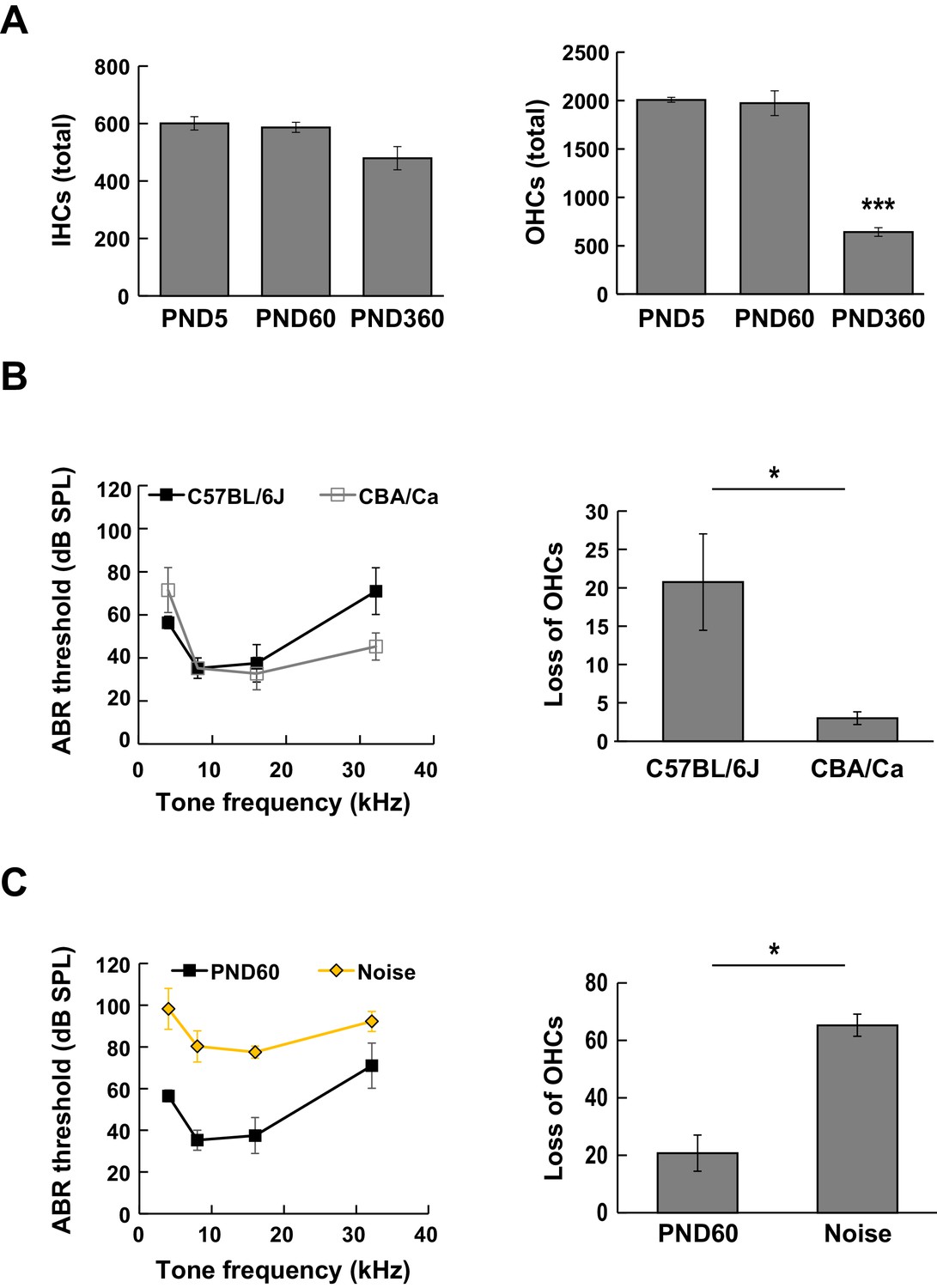
Manual counting of lost hair cells and auditory brainstem-evoked response (ABR) in mice with age-related and noise-induced hearing loss.
(A) Numbers of total IHCs and OHCs of C57BL/6J mice at PND 5, PND 60, and PND 360. (n = 4 (PND 5), 4 (PND 60), and 3 (PND 360). One-way ANOVA with Bonferroni's post hoc test, ***p < 0.001.) (B) ABR thresholds (left) and the numbers of lost OHCs (right) were compared between C57BL/6J (mouse model of age-related hearing loss) and CBA/Ca mice (control mice) at PND 60. (C) The effect of acoustic overexposure stimulus on ABR thresholds (left) and OHC loss (right) measured at PND 60. Acoustic overexposure stimulus induced an increase in ABR threshold and loss of OHCs. ABR, auditory brainstem response; IHC, inner hair cell; OHC, outer hair cell; PND, postnatal day.
Figure 2—figure supplement 2
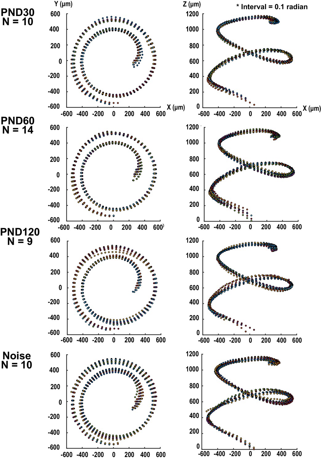
Three-dimensional presentation of hair cell distribution projected to X-Y and Y-Z planes.
Positions of Inner hair cells were sampled with regular intervals and the position data from different samples were overlaid. Hair cells from different samples were plotted as dots with different colors. Spiral directions of samples from right ears were converted to those of left ears for alignment of samples from both sides. PND, postnatal day.
Figure 3 with 1 supplement

Spatial pattern of hair cell loss.
(A) Pseudo-color presentation of hair cell loss along the longitudinal axis of the organ of Corti (PND 30, 60, and 120 and noise exposure at PND 60). Each row represents a single cochlear sample. Numbers of lost hair cells within 50 μm segments along the longitudinal axis were measured. For samples with higher cell loss in the basal portion, it was difficult to define the basal end of the sensory epithelium. These samples with ambiguous starting points of the epithelium were marked by thin red lines in rows of noise-exposed samples. The raw fluorescence image shows the definition of directions (distal and proximal, apex and base) relative to the sensory epithelium. (B) Distribution of lost cells along the longitudinal axis of the organ of Corti in three experimental groups. PND 60 and 120, and noise exposure at PND 60, exhibit distinct patterns of hair cell loss (Kruskal–Wallis test with Steel–Dwass test). (C) Detection of hair cell loss at the helicotrema. Scale bar, 100 μm. (D) Distribution of lost cells along the radial axis of the organ of Corti. Samples from PND 60 and 120 exhibit gradients of cell loss. (Paired t-test followed by Bonferroni’s correction, *p < 0.05; ***p < 0.001.) Number of samples; n = 10 (PND 30), 14 (PND 60), 9 (PND 120), and 10 (Noise), except for n = 7 in segment ‘a’ of Noise in (B). *p < 0.05; **p < 0.01; ***p < 0.001. PND, postnatal day.
-
Figure 3—source data 1
Source data for Figure 3D and Figure 3—figure supplement 1.
- https://doi.org/10.7554/eLife.40946.015
Figure 3—figure supplement 1
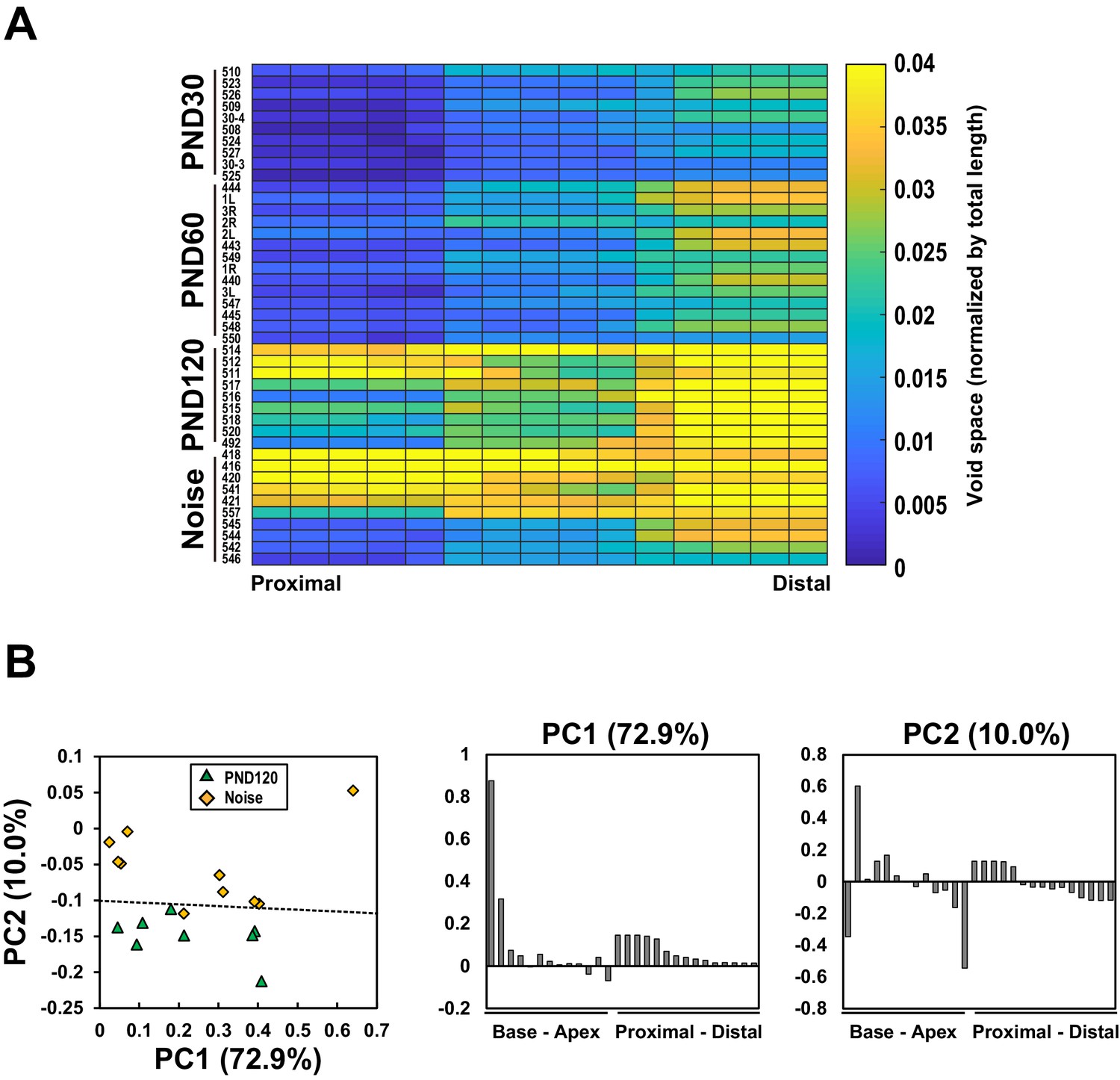
Longitudinal and radial distribution of hair cell loss in the organ of Corti.
(A) Pseudo-color presentation of the OHC loss frequency along the radial axis. Each row represents a single cochlear sample. The sample IDs were written on the left of the map. Note that the direction of comparison (proximal to distal) is perpendicular to the map shown in Figure 3A. Samples were arranged according to the extent of total cell loss in each experimental group from the highest to the lowest. The radial positions were divided into 15 sections and the scores were averaged within the sections. (B) Principal-component analysis (PCA) of the lost cell distribution in samples at PND 120 and at PND 60 with noise exposure (left). PCA was performed with the local OHC loss frequencies as variables. Frequencies of cell loss were calculated in individual segments set along the longitudinal and the radial axes. The percent variation explained by each principal component (PC) is indicated in parentheses. A dotted line indicates the decision boundary of the linear discriminant analysis. Coefficients of the first principal component (middle) and the second principal component (right) were presented from basal to apical and from proximal to distal. PND, postnatal day.
Figure 4 with 1 supplement
Model-based analysis of clustered cell loss.
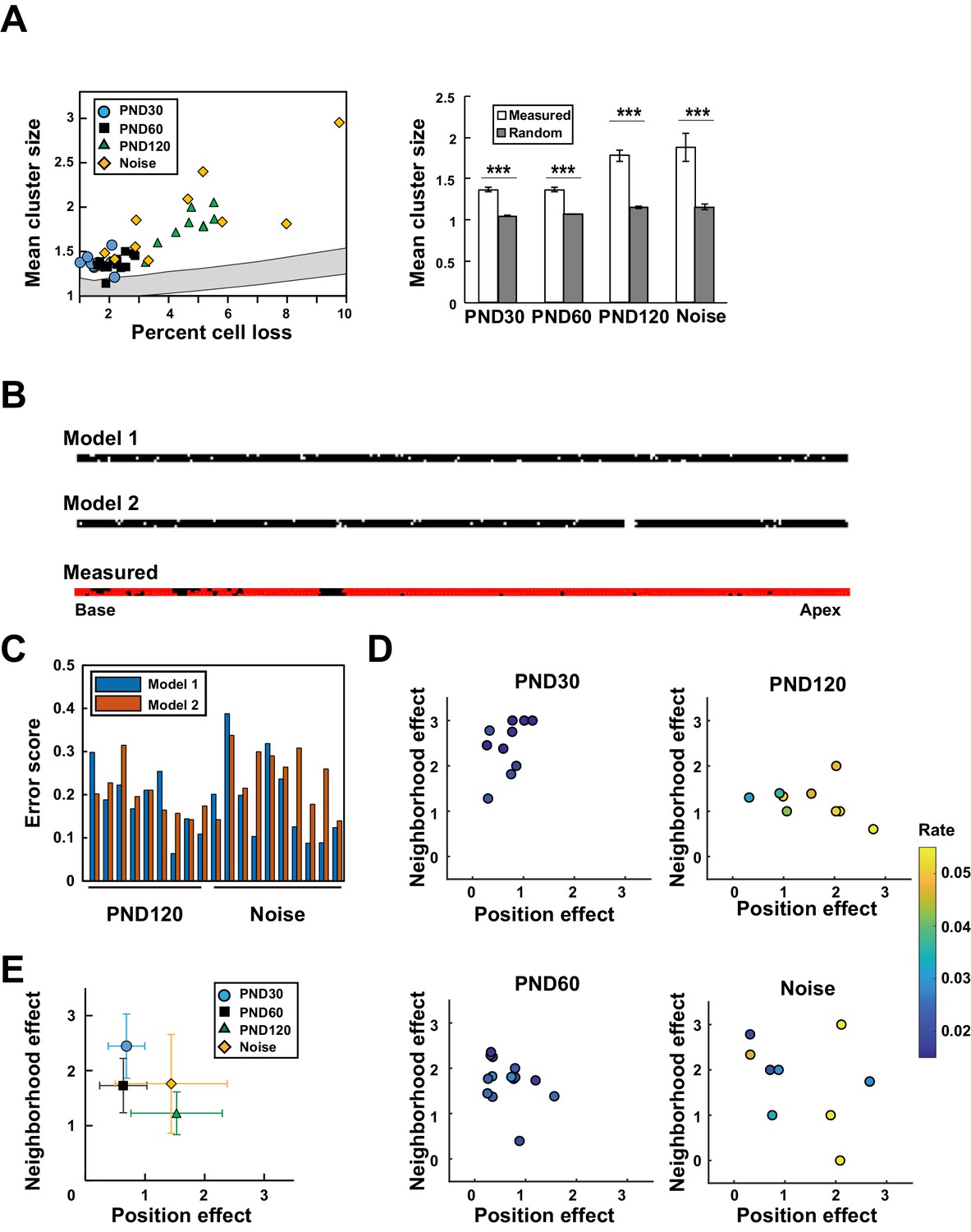
(A) Evaluation of the extent of clustered cell loss by comparison with the extent of clustering based on a model of random cell loss. The extent of cell clustering in the experimental data was much higher than would have been expected from random cell loss (99% confidence intervals within two lines) (Welch’s t-test, ***p < 0.001). (B) Construction of two models of hair cell loss (upper: neighborhood effect model; lower: position effect model). Virtual cell loss data were generated from the models and compared with the experimental data (measured). (C) Evaluation of the goodness-of-fit of the two models to the experimental data using the error score, which measures the extent of deviation of the clustering properties generated by the models from those observed in real samples. (D) Assessment of the relative contributions of the two models (neighborhood effect and position effect) to achieve the best fit to the experimental data. The two models contribute differentially under various conditions. The color code shows the proportion of lost OHCs against the total OHCs. (E) Overall pattern of contribution from two models. Note that the neighborhood effect makes a stronger contribution in young adult mice, whereas the position effect makes a stronger contribution in aged mice (means ± SD). Number of samples; n = 10 (PND 30), 14 (PND 60), 9 (PND 120), and 10 (Noise). PND, postnatal day.
-
Figure 4—source data 1
Source data for Figure 4A, C, D and E.
- https://doi.org/10.7554/eLife.40946.018
Figure 4—figure supplement 1
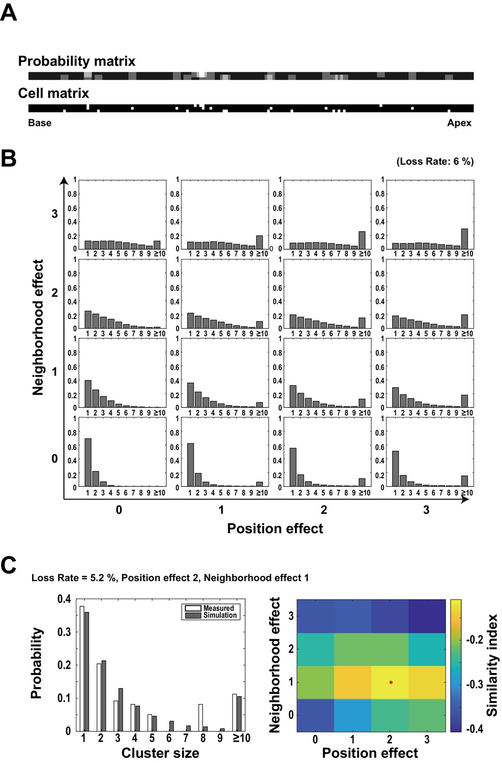
Simulation analysis of clustered cell loss.
(A) A pair of ‘probability matrix’ (upper panel) and ‘cell matrix’ (lower panel). The intensities of elements in the ‘probability matrix’ indicate the probability of cell loss for the next round of the simulation runs for individual cells. White pixels in the ‘cell matrix’ indicate the locations of already lost cells in previous rounds of the simulation runs. (B) An example of simulated histograms with different amounts of two effects (neighborhood effect and position effect). These histograms indicate the frequency distribution of cell loss clusters with different sizes. (C) Comparison of experimental data and simulation results for a given cochlear sample (No. 517). A heat map (right) shows the relative similarities between the experimental data and the simulation result (reverse of the error score in Figure 4C) when the weights of the neighborhood effect and the position effect were systematically changed. The weighted average point indicated by the red dot was taken as the estimated contributions of two effects to this sample.
Figure 5
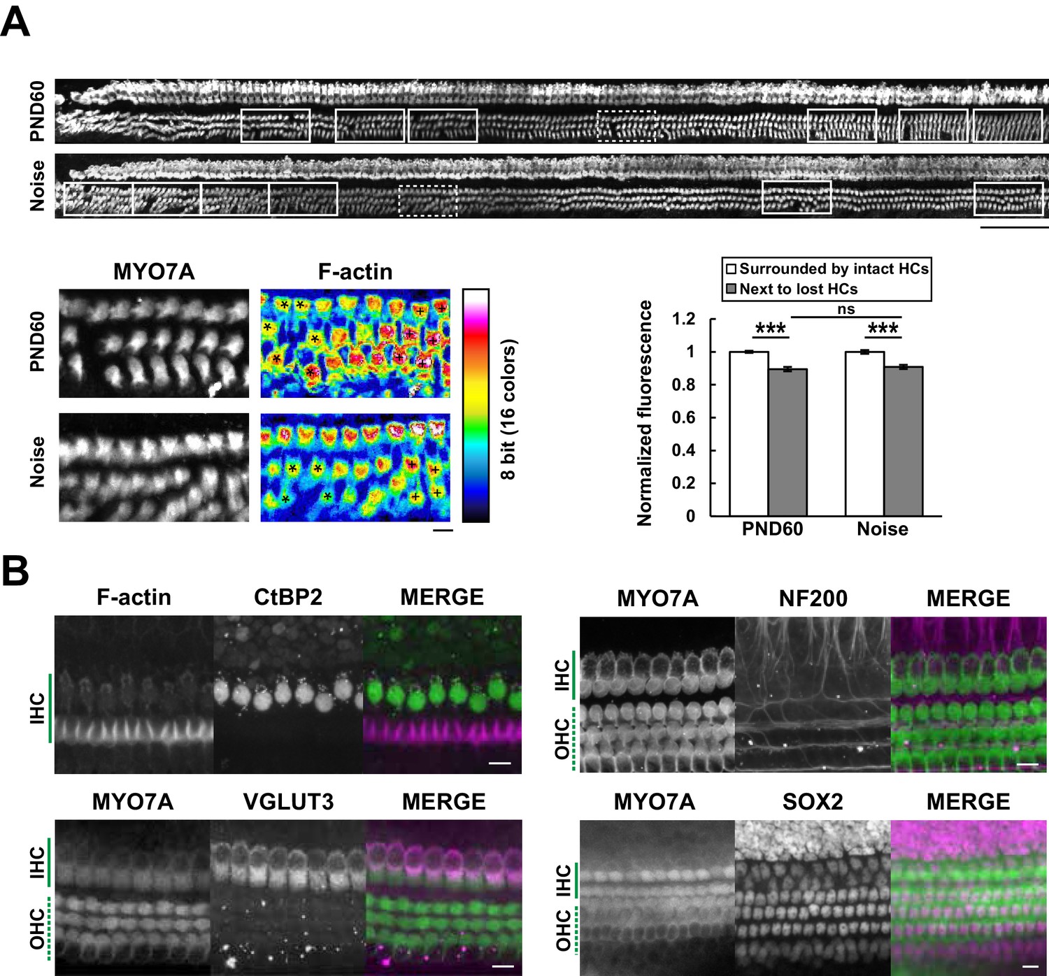
Efficient mapping of subcellular pathology and multiple cellular components.
(A) Automated detection of areas with variable degrees of hair cell loss, combined with evaluation of subcellular pathology. All sites of hair cell loss (white squares) were selected, and changes in the F-actin content were evaluated (upper image). White squares with dotted lines are representative analysis areas, and are enlarged at lower left. Hair cells surrounded by intact hair cells (crosses) or next to lost cells (asterisks) were compared for their F-actin content (lower right). The graph reveals loss of F-actin in hair cells adjacent to lost cells. Scale bars, 100 μm (upper) and 10 μm (lower). [n = 108 (PND 60) and 103 (Noise), paired t-test for comparison within the group, Welch’s t-test with Bonferroni’s correction for comparison of cell groups between different experimental conditions, ***p < 0.001; ns, not significant, p > 0.05.] (B) Modified ScaleS technique can be adapted to multiple immunohistochemistry of cellular and subcellular components at PND 5. Antibodies against CtBP2, VGLUT3, NF200, and SOX2 were used to detect multiple components in situ. Scale bars, 10 μm. HC, hair cell; IHC, inner hair cell; OHC, outer hair cell; PND, postnatal day.
-
Figure 5—source data 1
Source data for Figure 5A.
- https://doi.org/10.7554/eLife.40946.020
Appendix 2—figure 1

First the line passing through the centers of two images were generated, and the line passing through the center of the image overlap and perpendicular to the first line was created (the center line).
Distance of each pixel to the center line was defined as . The pixel that has the largest distance was selected and its value was normalized to be 1.
Appendix 2—Figure 2
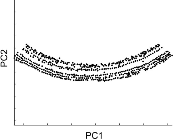
Distribution of intensity peaks within the plane of the first and second principal components.
The first principal component matched the longitudinal axis, while the second matched the radial axis.
Appendix 2—Figure 3
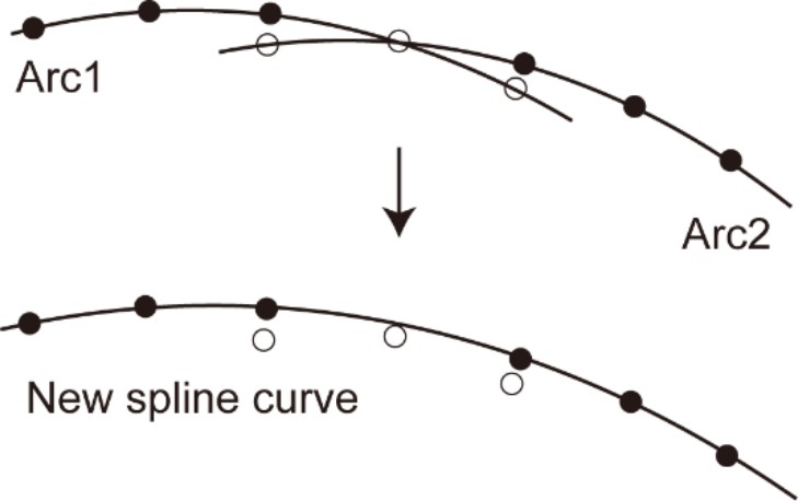
The method of stitching two arcs.
Among the dots on the two arcs, the open dots were removed and the closed dots were fitted with a spline curve.
Appendix 2—figure 4
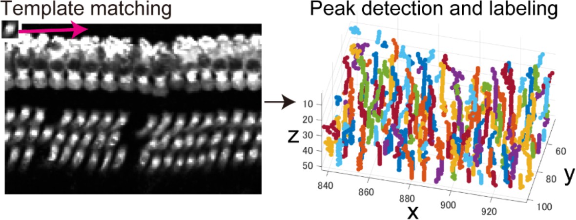
Extraction of cell candidates by template matching.
Left; Template matching with the small template image (upper left) was performed for individual x-y images within the image stack. Right; Detection and labeling of correlation peaks distributed within three-dimensional matrix generated by calculation of cross-correlation. Cell candidates were assemblies of correlation peaks grouped by connected-component labeling.
Appendix 2—figure 5

Functions of the third and fourth machine learning models.
Cell candidates detected by the first and the second machine learning models were further categorized into three rows by the third model (cells marked by dots with different colors correspond to the three rows.). The spaces between detected OHCs (asterisks) were detected and evaluated the possible presence of OHCs escaped in the previous detection processes.
Appendix 2—figure 6

Comparison of detection efficiencies between a standard image processing method and our method (Paired t-test, both p < 0.0001, n = 10 linearized whole cochlear images).
https://doi.org/10.7554/eLife.40946.030
Appendix 2—figure 7

Comparison of 3D watershed and our machine learning based method.
There are many duplicate count and false detection with 3D watershed method.
Appendix 2—figure 8
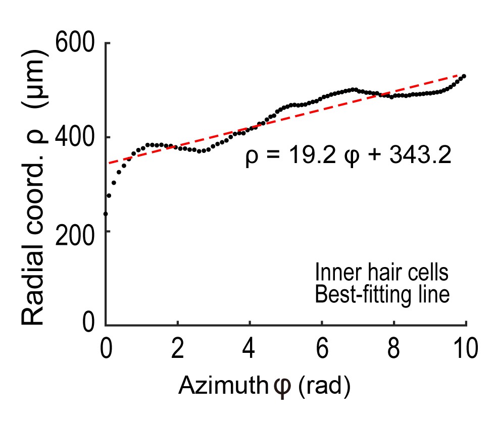
An example of fitting the increasing distance between IHCs and the modiolus to a smooth spiral.
The line with the minimum sum of squared errors was chosen to be the longitudinal axis of the cylindrical coordinate system.
Appendix 2—figure 9

An example of inner hair cell locations (black dots) viewed from the axial direction.
The angle () was measured from the line (red line) connecting the center of the spiral and the inner hair cell located at the end of the apex (green dot).
Appendix 2—figure 10
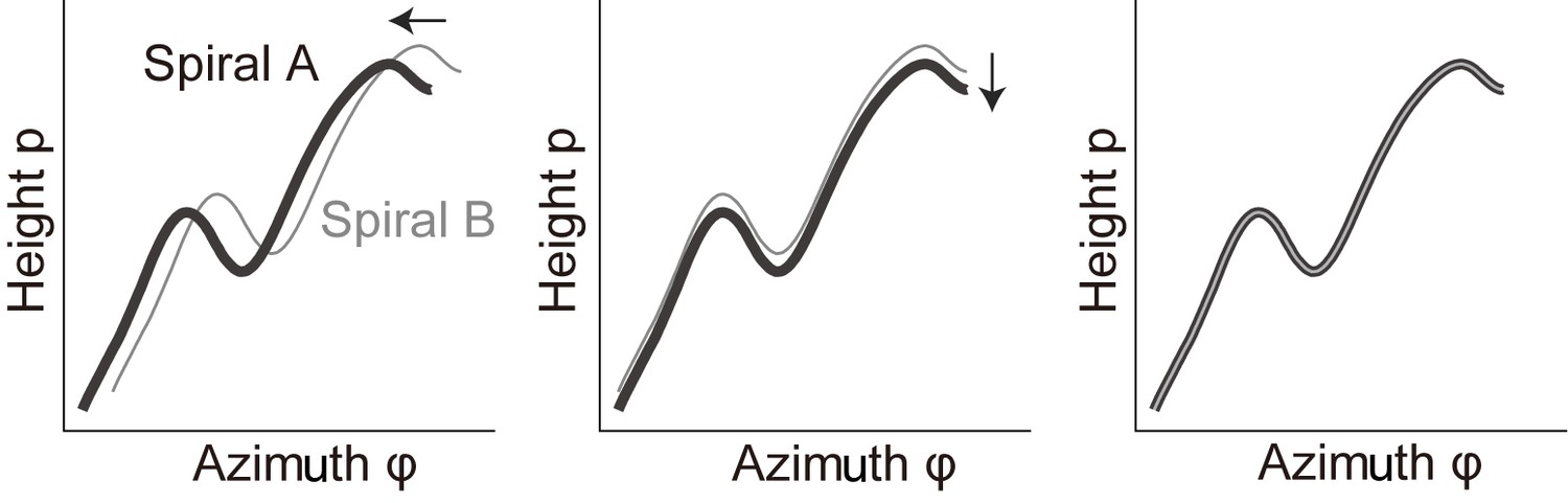
Evaluation of the extent of correlation between two curves in the plane of -.
Within this plane, the positions of spiral A and B were aligned. First, the shift in was adjusted (middle). Subsequently, the shift in was adjusted (right).
Appendix 2—figure 11
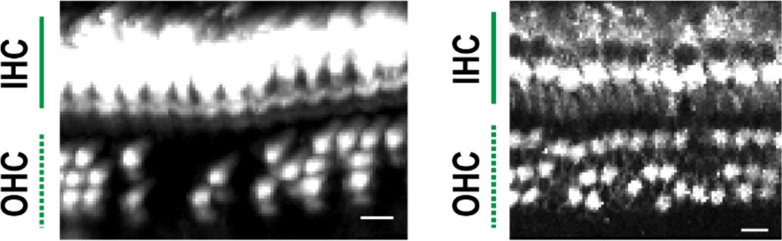
Representative examples of hair cell images where manual estimation of cell loss was difficult.
The number of lost cells is difficult to estimate when the size of cell-negative area increases in the basal turn (left). Disorganized rows of OHCs were frequently observed in the apical turn (right). Identification of lost cell positions is difficult when cell density is not high enough to estimate the rows (left) or cells are not aligned as horizontal rows (right). Scale bars, 10 μm.
Appendix 2—figure 12
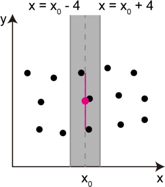
Procedures of obtaining parameters necessary for radial alignment (along y-axis) of cell centers.
Calculation of an averaged y position of the cell group (a red circle) and a vertical spread of the cell group (a red vertical line). These two parameters were calculated in the area (colored in gray) containing more than two ‘cell centers’. Black dots indicate the positions of ‘cell centers’, and the variable x0 indicates the x-coordinate of the averaged cell center within the gray area.
Appendix 2—figure 13
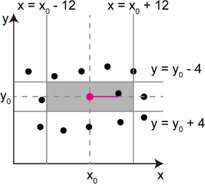
Procedures of obtaining parameters necessary for longitudinal alignment (along x-axis) of cell centers.
Calculation of the horizontal distance between adjacent cells (red horizontal line). The nearest cell in the rectangular area (colored in gray) was selected for the calculation. The variables x0 and y0 are the coordinates of the parental cell center (red dot).
Tables
Table 1
Details of machine learning models (related to Figure 2).
https://doi.org/10.7554/eLife.40946.010| Models | Type‡ | Algorithm | Configuration | Use | Predictor |
|---|---|---|---|---|---|
| IHC* 1 | Binary | Gentle Boost | 300 classification trees | Reduction of noise | Area, barycentric coordinates, maximum correlation coefficients, maximum intensity, same data set of the nearest neighbor group and relative position of the nearest neighbor group |
| IHC* 2 | Binary | Random Forest | 300 classification trees | Detection of cells | Adding to the above, prediction score by ‘IHC* 1’ of itself and that of adjacent groups in six directions¶, relative position of the adjacent groups, and cropped image†† |
| OHC† 1 | Binary | Gentle Boost | 300 classification trees | Reduction of noise | Same as ‘IHC* 1’ |
| OHC† 2 | Binary | Random Forest | 300 classification trees | Detection of cells | Same as ‘IHC* 2’ |
| OHC† 3 | Multiclass | Convolutional Neural Network | From the input, convolutional layer (filter size 5, number 60), ReLU§ layer, fully connected layer, Softmax Layer (three classes), and output. | Estimation of belonging row | Cropped image (39 × 69 pixels in width and height) |
| OHC† 4 | Binary | Convolutional Neural Network | From the input, convolutional layer (filter size 5, number 60), ReLU§ layer, convolutional layer (filter size 5, number 20), ReLU§ layer, fully connected layer, Softmax Layer (two classes), and output. | Detection of cells in spaces | Cropped image (39 × 69 pixels in width and height) |
-
*. IHC, inner hair cell.
†. OHC, outer hair cell.
-
‡. Classification type.
§. Rectified Linear Unit.
-
¶. Adjacent groups in direction of 0–60°, 60–120°, 120–180°, 180–240°, 240–300°, 300–360° with the y-axis as an initial line in the x-y plane.
††. Initial image size is 21 × 69 pixels in width and height. The image is resized in 7 × 23 then reshaped in 1 × 161.
Table 2
Detection efficiency of hair cells (related to Figure 2).*
https://doi.org/10.7554/eLife.40946.011Inner hair cell | |||||
|---|---|---|---|---|---|
| Detect. (n)† | Undetect. (n)‡ | Err. detect. (n)§ | Recover Rate¶ | Accuracy rate†† | |
| Our Method | 576 ± 33 | 13 ± 12 | 2 ± 2 | 0.979 ± 0.021 | 0.997 ± 0.003 |
| 3D Watershed | 424 ± 98 | 152 ± 82 | 110 ± 78 | 0.733 ± 0.149 | 0.818 ± 0.100 |
| Outer hair cell | |||||
| Detect. (n)† | Undetect. (n)‡ | Err. Detect. (n)§ | Recover Rate¶ | Accuracy rate†† | |
| Our Method‡‡ | 1989 ± 133 | 24 ± 13 | 6 ± 4 | 0.988 ± 0.006 | 0.997 ± 0.002 |
| Principle 1 Only§§ | 1925 ± 131 | 69 ± 41 | 16 ± 13 | 0.966 ± 0.021 | 0.992 ± 0.006 |
| 3D Watershed | 1493 ± 197 | 496 ± 111 | 760 ± 381 | 0.748 ± 0.064 | 0.682 ± 0.103 |
-
*. Data from 10 samples (PND30: two sample, PND60: three sample, ACL: two sample, NCL: three sample). Data are expressed as means ± SD.
†. Detection number.
-
‡. Undetected number.
§. Erroneous detection number.
-
¶. Recover rate of manually identified hair cells by the automated detection algorithm (almost synonymous with recall).
††. The number of hair cells identified by both manual and automated detection divided by the number of hair cells identified by automated detection (almost synonymous with precision).
-
‡‡.The proposed method in this study (principle 1 + principle 2).
§§. The method using the first half of the proposed method. For details please see ‘Principles of auto-detection by machine learning’ in Appendix 2.
Table 3
Inter-operator percent match in void space detection (related to Experimental procedures).
https://doi.org/10.7554/eLife.40946.012| Inter-operator percent match | Number of detected void space | ||||||
|---|---|---|---|---|---|---|---|
| Sample number | A¶-B¶ | B¶-C¶ | A¶-C¶ | Auto††-HC‡‡ | Both | Auto††-only | HC‡‡-only |
| 1* | 0.960 | 0.880 | 0.917 | 0.920 | 24 | 1 | 1 |
| 2† | 0.898 | 0.917 | 0.906 | 0.952 | 84 | 2 | 2 |
| 3‡ | 0.923 | 0.885 | 0.958 | 0.889 | 24 | 3 | 0 |
| 4§ | 0.923 | 0.882 | 0.846 | 0.926 | 50 | 3 | 1 |
| Overall | 0.916 | 0.898 | 0.897 | 0.931 | 182 | 9 | 4 |
-
*. Sample 1, two months old, total loss rate of OHCs: 1.7%.
†. Sample 2, two months old with noise exposure, total loss rate of OHCs: 8.1%.
-
‡. Sample 3, one month old, total loss rate of OHCs: 2.2%.
§. Sample 4, four months old, total loss rate of OHCs: 4.2%.
-
¶. Skilled human operators (A, B, and C).
††. Auto, automated OHC loss counting program.
-
‡‡. HC, human consensus.
Key resources table
| Reagent type (species) or resource | Designation | Source or reference | Identifiers | Additional information |
|---|---|---|---|---|
| Genetic reagent (M. musculus) | C57BL/6J | Sankyo Lab (JAPAN) | PRID:MGI:5658686 | |
| Genetic reagent (M. musculus) | CBA/Ca | Sankyo Lab (JAPAN) | PRID:MGI:2159826 | |
| Genetic reagent (M. musculus) | Thy1-GFP line-M | Jackson Lab | PRID:MGI:3766828 | |
| Genetic reagent (M. musculus) | GO-Ateam | PMID: 19720993 | Dr. M Yamamoto (Kyoto University, Japan) | |
| Antibody | Rabbit polyclonal anti- Myosin VIIa | Proteus Biosciences | cat# 25–6790 PRID:AB_10013626 | IHC (1:100) |
| Antibody | Mouse monoclonal anti-Neurofilament 200 | SIGMA | cat# N5389 PRID:AB_260781 | IHC (1:100) |
| Antibody | Mouse monoclonal anti-SOX-2 | EMD Millipore | cat# MAB4343 PRID:AB_827493 | IHC (1:200) |
| Antibody | Mouse monoclonal anti-CTBP2 | BD Bioscience | cat# 612044 PRID:AB_399431 | IHC (1:100) |
| Antibody | Guinea pig polyclonal anti-VGLUT3 | PMID: 20034056 | IHC (1:500), Dr. H Hioki (Juntendo University, Japan) | |
| Antibody | Alexa Fluor 488-conjugated mouse monoclonal anti-VE cadherin | eBioscience | cat# 16-1441-81 PRID:AB_15604224 | IHC (1:500) |
| Chemical compound, drug | Rhodamine phalloidin | Invitrogen | cat# R415 | IHC (1:500) |
| Chemical compound, drug | Triton X-100 | Nakalai-tesque | cat# 12967–45 | |
| Chemical compound, drug | Urea | SIGMA | cat# U0631-1KG | |
| Chemical compound, drug | N,N,N',N'-Tetrakis (2-eydroxypropyl) ethylendiamine | TCI | cat# T0781 | |
| Chemical compound, drug | D-sucrose | Wako | cat# 196–00015 | |
| Chemical compound, drug | 2,2',2''-nitrilotriethanol | Wako | cat# 145–05605 | |
| Chemical compound, drug | Dichloromethane | SIGMA | cat# 270997–100 ML | |
| Chemical compound, drug | Tetrahydrofuran | SIGMA | cat# 186562–100 ML | |
| Chemical compound, drug | Dibenzyl Ether | Wako | cat# 022–01466 | |
| Chemical compound, drug | Methanol | Wako | cat# 132–06471 | |
| Chemical compound, drug | D-glucose | SIGMA | cat# G8270-100G | |
| Chemical compound, drug | D-sorbitol | SIGMA | cat# S1816-1KG | |
| Chemical compound, drug | Thiodiethanol | Wako | cat# 205–00936 | |
| Chemical compound, drug | Acrylamide | Wako | cat# 011–08015 | |
| Chemical compound, drug | Bis-acrylamide | SIGMA | cat# 146072–100G | |
| Chemical compound, drug | VA-044 initiator | Wako | cat# 225–02111 | |
| Chemical compound, drug | Sodium dodecyl sulfate | TCI | cat# I0352 | |
| Chemical compound, drug | FocusClear | CelExplorer Labs | cat# F101-KIT | |
| Chemical compound, drug | Glycerol | Wako | cat# 075–00616 | |
| Chemical compound, drug | Dimethyl sulfoxide | Wako | cat# 043–07216 | |
| Chemical compound, drug | N-acetyl-L-hydroxyproline | TCI | cat# A2265 | |
| Chemical compound, drug | Methyl-β-cyclodextrin | TCI | cat# M1356 | |
| Chemical compound, drug | γ-cyclodextrin | TCI | cat# C0869 | |
| Chemical compound, drug | Tween-20 | Wako | cat# 167–11515 | |
| Software, algorithm | ImageJ | NIH | PRID: SCR_003070 | |
| Software, algorithm | GraphPad Prism 6 | GraphPad Software | PRID: SCR_002798 | |
| Software, algorithm | MATLAB | MathWorks | PRID: SCR_001622 | |
| Software, algorithm | Microsoft Excel | Microsoft | PRID: SCR_016137 | |
| Software, algorithm | Adobe Illustrator | Adobe | PRID: SCR_010279 | |
| Software, algorithm | Signal processor | Nihon Kouden | Neuropack MEB2208 | |
| Other | MATLAB codes | This paper | https://github.com/okabe-lab/cochlea-analyzer | |
| Other | 25x water- immersion objective lens | Nikon | N25X-APO-MP | |
| Other | 25x water- immersion objective lens | Olympus | XPLN25XWMP | |
| Other | Sound speaker | TOA | HDF-261–8 | |
| Other | Power amplifier | TOA | IP-600D | |
| Other | Condenser microphone | RION | UC-31 and UN14 | |
| Other | Sound calibrator | RION | NC-74 | |
| Other | Noise generator | RION | AA-61B | |
| Other | Dual channel programmable filter | NF corporation | 3624 |
Table 4
Number of training and test dataset, and performance evaluation of machine learning models (related to Figure 2).
https://doi.org/10.7554/eLife.40946.021| Model | Training | Test | Recall | Precision | F score | ||
|---|---|---|---|---|---|---|---|
| Total (n) | Positive labels (n) | Total (n) | Positive labels (n) | ||||
| IHC* 1 | 607,954 | 5906 | 578,851 | 5741 | 0.961 | 0.941 | 0.951 |
| IHC* 2 | 37,576 | 11,977 | 18,104 | 5753 | 0.977 | 0.986 | 0.981 |
| OHC† 1 | 1,112,659 | 20,576 | 1,099,519 | 19,959 | 0.978 | 0.914 | 0.945 |
| OHC† 2 | 28,702 | 20,576 | 27,185 | 19,959 | 0.959 | 0.979 | 0.969 |
| OHC† 3 | 20,416 | Row1: 6706 Row2: 6745 Row3: 6965 | 19,594 | Row1: 6421 Row2: 6450 Row3: 6723 | 0.993‡ | 0.993‡ | 0.993‡ |
| OHC† 4 | 4114 | 1365 | 2990 | 905 | 0.920 | 0.946 | 0.933 |
-
*. IHC, inner hair cell.
†. OHC, outer hair cell.
-
‡. Calculated by micro-average of recall and precision (Sokolova M and Lapalme G, 2009)
Additional files
-
Transparent reporting form
- https://doi.org/10.7554/eLife.40946.022
Download links
A two-part list of links to download the article, or parts of the article, in various formats.
Downloads (link to download the article as PDF)
Open citations (links to open the citations from this article in various online reference manager services)
Cite this article (links to download the citations from this article in formats compatible with various reference manager tools)
Cellular cartography of the organ of Corti based on optical tissue clearing and machine learning
eLife 8:e40946.
https://doi.org/10.7554/eLife.40946


