Figures and data in Spatiotemporal establishment of dense bacterial colonies growing on hard agar | eLife

Figures
Additional files

22 figures and 1 additional file

Figures

Figure 1 with 1 supplement

Download asset Open asset

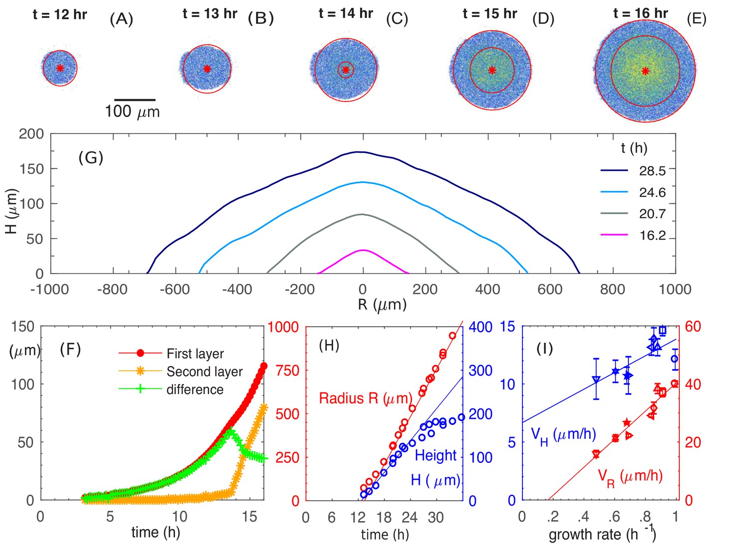
Experimental observations of the growth and morphology of a bacterial colony.

(A–E) Confocal images of an E. coli colony harboring GFP expression growing on 1.5% agar (glucose minimal medium) taken at various time after seeding ( $t = 0$ ). The center of the colony is indicated by the red dot. Single- and multi-layer regions are distinguished by red circles based on fluorescence intensity; see 'Experimental Methods'. (F) The radius of the first (red) and second layer (orange) of the colony, as well as their difference (green), versus time. (G) The cross-sectional profile of the growing bacterial colony at indicated time after single-cell inoculation. (H) After the buckling at around $t = 13$ h, the colony radius (red symbols) increased at a constant speed $V_{R} = 45.2 μ m / h$ (red line), while the colony height (blue symbols) increased linearly with speed $V_{H} = 12.4 μ m / h$ (blue line). The latter slowed down some time after $t = 24 h$ . (I) The dependence of the radial speed $V_{R}$ (red symbols) and the vertical speed $V_{H}$ (blue symbols) on cell growth rate (x-axis), for colonies grown in minimal medium with 8 different carbon sources (Supplementary file 1-Table S1): glucose (O); arabinose (□); mannitol ( $△$ ); maltose (◇); fructose ( $◃$ ); melibiose ( $▹$ ); sorbitol ( $▽$ ); mannose (☆). The lines are best linear fit of the data.

https://doi.org/10.7554/eLife.41093.002

Figure 1—source data 1 Experimental data for the temporal development of colony profiles and velocities.: https://doi.org/10.7554/eLife.41093.005
Download elife-41093-fig1-data1-v1.xlsx

Figure 1—figure supplement 1

Download asset Open asset

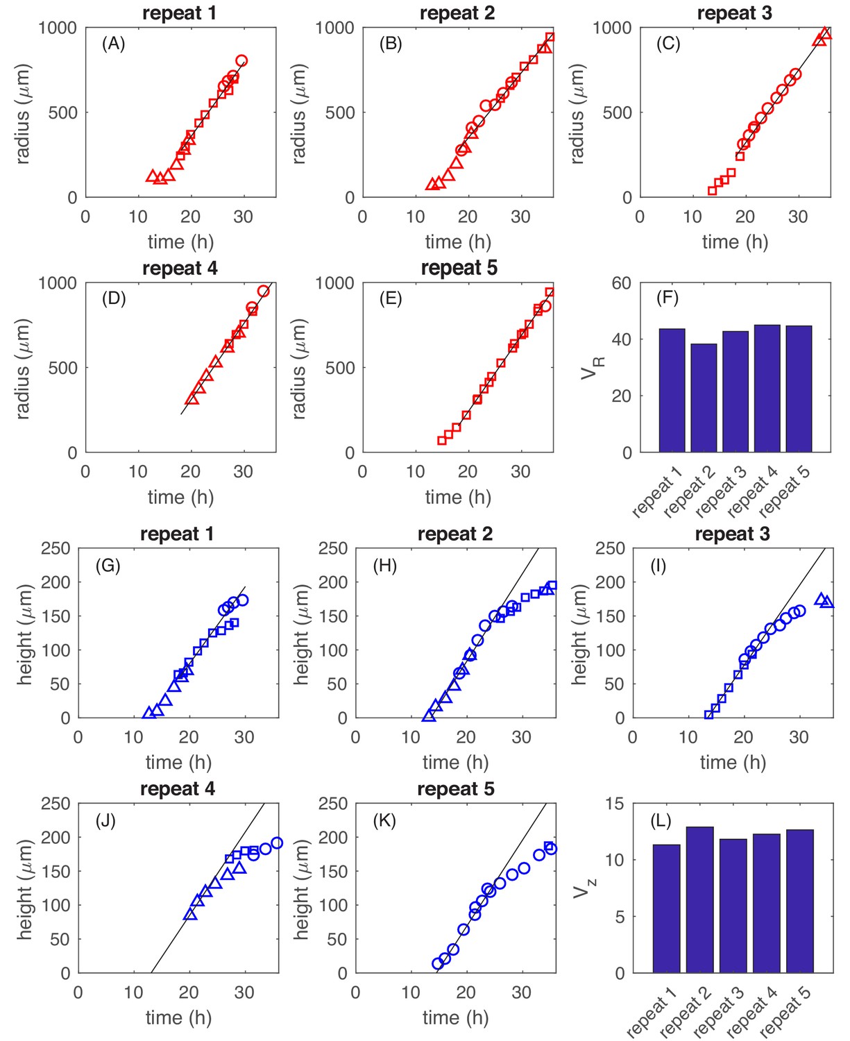
Data for five repeats of E.coli EQ59 grown on 1.5% (w/v) agar in minimal medium with 0.2% glucose (11 mM), and incubated, covered, at 37°C for up to 3 days; cf. 'Experimental Methods'.

Their radii and heights were periodically monitored using a confocal microscope. To monitor the colony growth over long periods of time, we started with identical colonies at seed time separated by several hours. Growth curves extending over a period of multiple days were obtained by 'stitching together' the radii and height data at times where they overlapped; cf. section on Experimental Methods. The recorded radii data (A)-(E) and height data (G)-(K) clearly showed linear regimes. The data were fitted by straight lines over the linear regimes to obtain the speed of radial expansion $V_{R}$ (F) and that of the height increasing $V_{H}$ (L) for these five repeated experiments. $V_{R}$ has an average of $42.84 μ m / h$ and standard deviation of $2.42 μ m / h$ . $V_{H}$ has an average of $12.18 μ m / h$ and standard deviation of $0.56 μ m / h$ . Similar analyses were done for colonies grown in other carbon sources described in Figure 1I.

https://doi.org/10.7554/eLife.41093.003

Figure 1—figure supplement 1—source data 1 Repetitions for the temporal development of colony height and radius.: https://doi.org/10.7554/eLife.41093.004
Download elife-41093-fig1-figsupp1-data1-v1.xlsx

Figure 2

Download asset Open asset

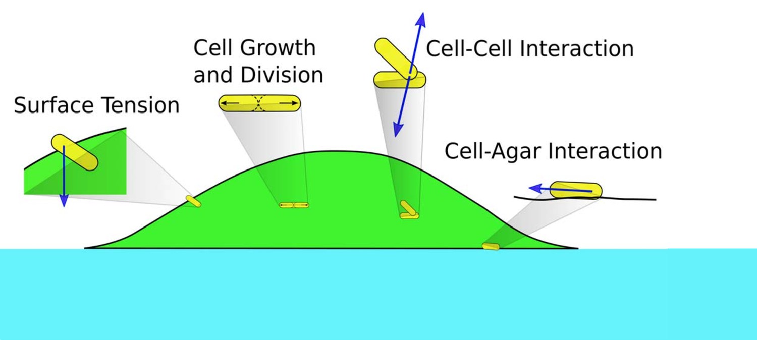
Schematics of cell-cell, cell-agar, cell-fluid, and surface tension forces investigated in this study.

Green area indicates the colony (with cells in yellow). Blue area indicates the agar.

https://doi.org/10.7554/eLife.41093.006

Figure 3 with 1 supplement

Download asset Open asset

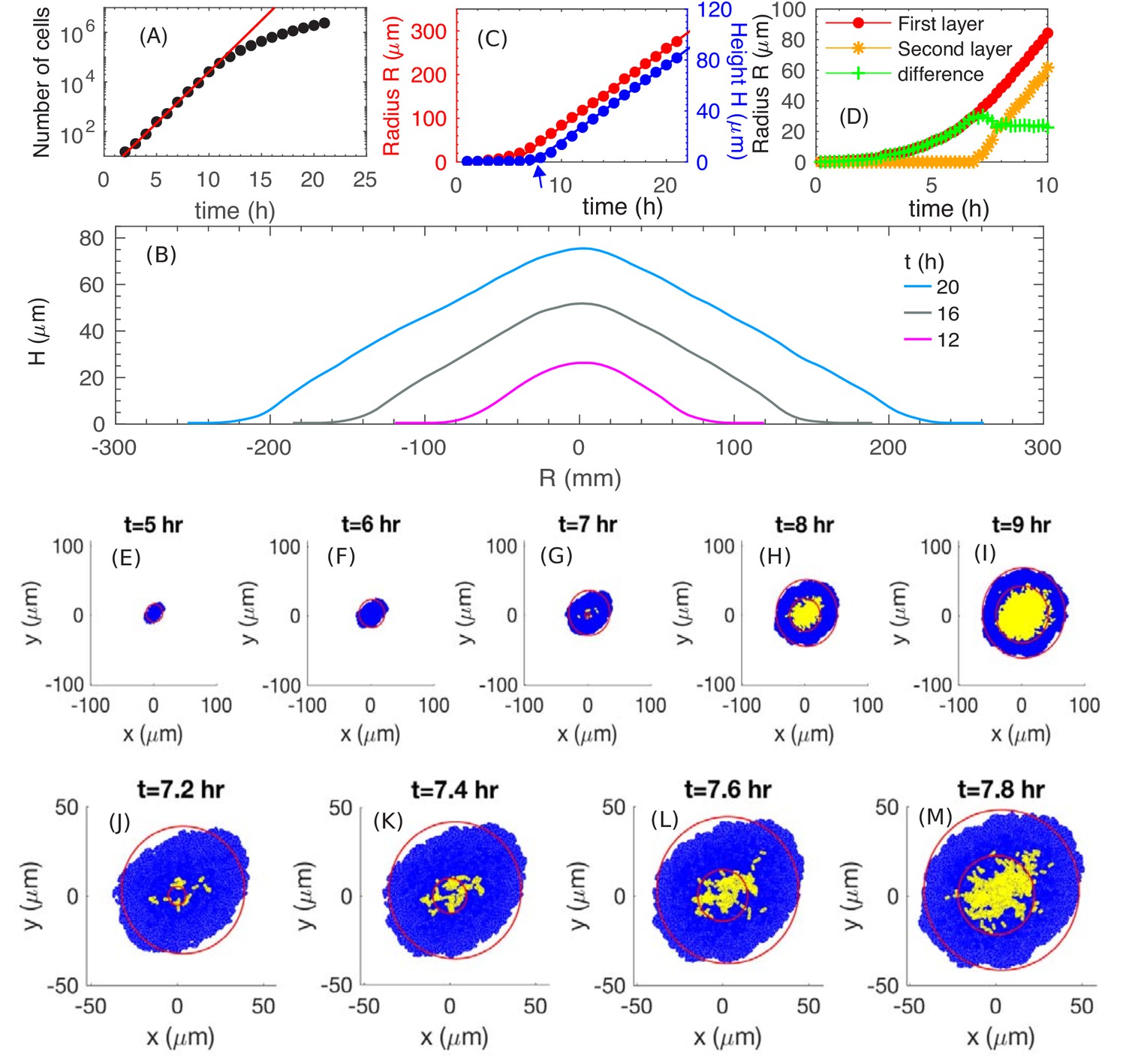
The simulated growth and morphology of a bacterial colony.

(A) A semi-log plot of number of cells vs. time showing the exponential growth of the population starting from a single cell at $t = 0$ . Red line shows exponential growth rate of $0.96 h^{- 1}$ . (B) Cross sections of the growing colony at various times after seeding of a single cell. (C) Plots of the radius (red) and height (blue) vs. time up to $t = 20 h$ , showing that, after an initial transient period of ~10 h, the growing colony increases linearly at the radial speed $V_{R} \approx 18 μ m / h$ (red line) and vertical speed $V_{H} \approx 6.0 μ m / h$ . The blue arrow at $t = 6 h$ indicates the time when the colony height starts to increase. (D) The radius of the first (red) and second (orange) layer of the colony as well as their difference (green) vs. time. (E–M) Top view of the colony at various time. Cells in the bottom layer (blue) and upper layers (yellow) are fitted into red circles. The time evolution of buckling phenomenon is captured in detail in (J–M).

https://doi.org/10.7554/eLife.41093.007

Figure 3—figure supplement 1

Download asset Open asset

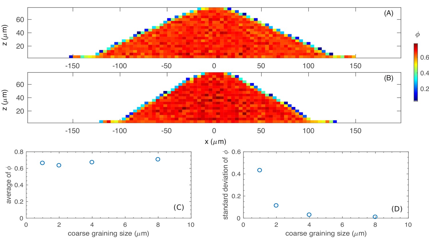
The spatially varying cell density $ρ$ (per unit volume of colony) is related to the spatially varying cell volume fraction $ϕ$ by $ρ = ϕ ρ_{c e l l}$ , where the volume fraction $ϕ$ is defined as the volume of all cells in a unit volume of the colony and $ρ_{c e l l}$ is the constant mass density of a typical mature cell; cf. Appendix 1.2 on nutrient update.

(A) and (B): The volume fraction $ϕ$ in the $x z$ cross section of the colony, calculated with the mean $m$ and standard deviation $σ$ , with (A) $λ_{S} = 1.0 h^{- 1}$ , $m = 0.678$ , and $σ = 0.030$ ; and (B) $λ_{S} = 0.5 h^{- 1}$ , $m = 0.680$ , and $σ = 0.034$ . (C) and (D): The effect of coarse-graining size to the volume fraction $ϕ$ . The average of $ϕ$ (C) and the standard deviation of $ϕ$ (D) in the coarse-graining with different sizes.

https://doi.org/10.7554/eLife.41093.008

Figure 4 with 2 supplements

Download asset Open asset

The cross-sectional anatomy of a simulated colony.

(A) Snapshot of cross-sectional view of the colony at $t = 20 h$ . Cyan represents horizontally oriented cells ( $\geq 45^{o}$ with z-axis); Yellow represents vertically oriented cells ( $\leq 45^{o}$ with z-axis). (B) Fraction of vertically oriented cells averaged over $z$ vs radius. (C) A side view of the azimuthally averaged director field, indicating the orientation of the rod-like cells. (D) A side view of the azimuthally averaged velocity field. (E) Vertical component of velocity, $V_{z}$ , at various values of $z$ along the center of the colony. Increase in vertical speed is seen only for the bottom 10 µm (F) A cross-sectional view of the colony, color representing the time since last division. Purple and blue represent cells that have not divided for the past 10 h, and red represents the actively dividing cells. (G) A cross-sectional view of the local growth rate in the colony, with the color bar showing the values of local growth rate. A disc-shaped 'growth zone' is revealed by the red color at the bottom of the colony.

https://doi.org/10.7554/eLife.41093.009

Figure 4—figure supplement 1

Download asset Open asset

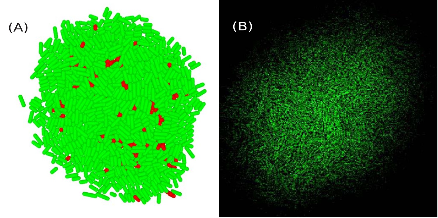
A few top layers of cells in the colony visualized using simulation data.

(A) and experimental data (B). In (A), a cell is colored green (resp. red) if its angle with the vertical $z$ -axis is less (resp. greater) than $45^{\circ}$ .

https://doi.org/10.7554/eLife.41093.010

Figure 4—figure supplement 2

Download asset Open asset

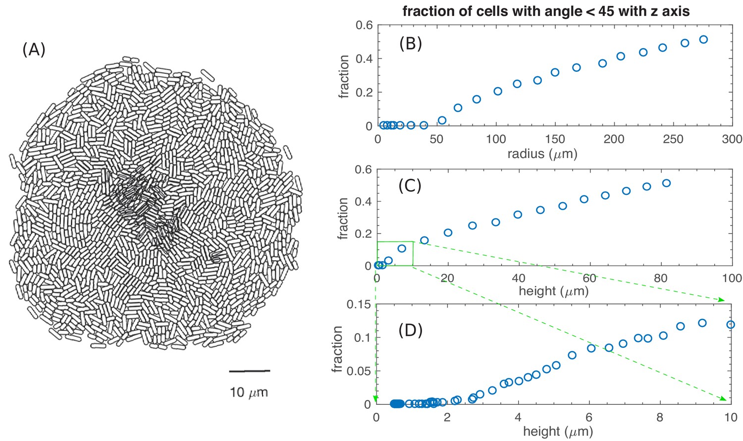
Fraction of verticalized cells increase for large colonies.

(A) The bottom view of a simulated colony at $t = 7 h$ , with the cells outlined by the black curves. Overlapping cells are of different layers. (B)-(D) show the fraction of vertically oriented cells (cells with an angle $< 45^{o}$ with $z$ axis) plotted versus the radius of the colony (B), the height of the colony up to 80 µm (C), and the height of the colony up to 10 µm (D).

https://doi.org/10.7554/eLife.41093.011

Figure 5 with 2 supplements

Download asset Open asset

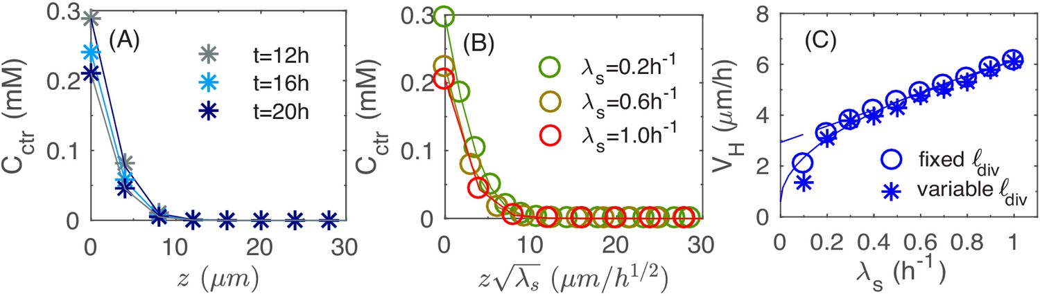
Vertical penetration of nutrients.

(A) The profiles of nutrient concentration $C_{c t r} (z) = C (0,0, z)$ along the z-axis at different times. (B) The profile $C_{c t r} (z)$ in the uniform scale vs. that in the rescaled z-axis, $z \sqrt{λ_{S}}$ . (C) The numerical results for the height velocity $V_{H}$ vs. the batch culture growth rate $λ_{S}$ with a fixed cell division length $l_{d i v}$ (open circles) and variable $l_{d i v}$ (asterisk), respectively. The square root fit for the open circles (solid line) is given by the expression $V_{H} = 5.5 \sqrt{λ_{S}} + 0.6$ ; the linear fit for circles with $λ_{S} \geq 0.5 h^{- 1}$ (dashed line) is given by the expression $V_{H} = 3.2 λ_{S} + 2.9$ .

https://doi.org/10.7554/eLife.41093.012

Figure 5—figure supplement 1

Download asset Open asset

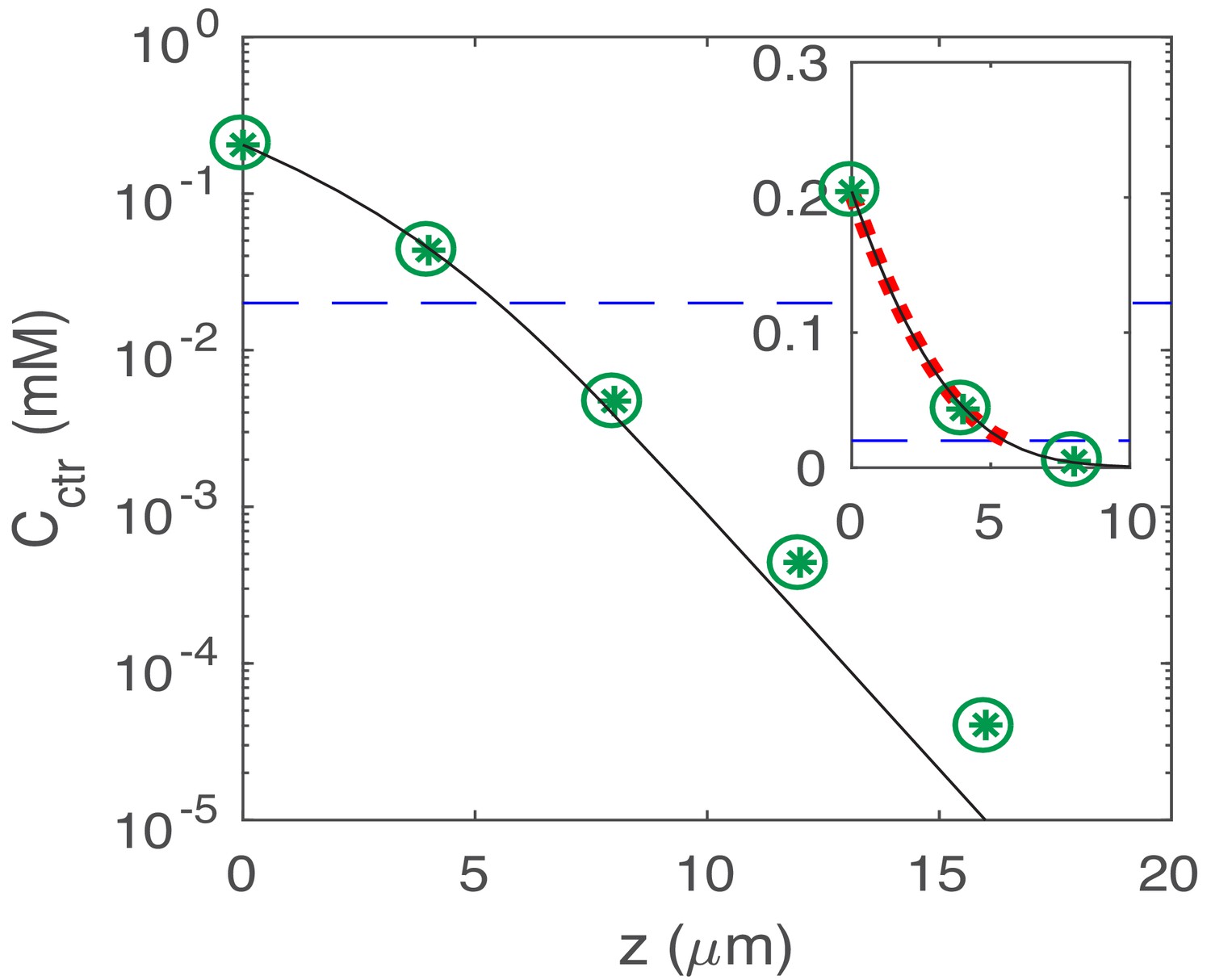
Semi-log plot of the steady-state nutrient profile $C_{c t r} (z) = C (0, 0, z)$ : reconstructed from 3D simulations (green *); and the numerical solution to the 1D model (cf. Appendix 2.3 on nutrient penetration) with discretization $Δ z = 4 μ m$ (green circles) and $Δ z = 0.1 μ m$ (black line), respectively.

The linear part below the line of the Monod constant $K_{S} = 0.02 m M$ (dashed blue line) indicates the exponential decay of the concentration. Shown in the window is the quadratic curve $C_{c t r} (z) = {(0.0663 z - 0.433)}^{2} + 0.016$ (red dotted line), fitting the numerical solution to the 1D model with $Δ z = 0.1 μ m$ for the concentration value above the Monod constant.

https://doi.org/10.7554/eLife.41093.013

Figure 5—figure supplement 2

Download asset Open asset

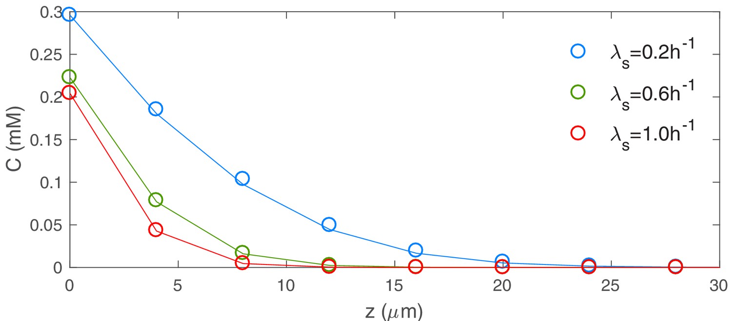
Profiles of nutrient concentration $C_{c t r} (z) = C (0,0, z)$ versus $z$ for various values of the batch culture growth rate $λ_{S}$ .

These nutrient profiles were reconstructed from 3D simulations. A larger value of the batch culture growth rate $λ_{S}$ leads to a lower nutrient concentration, indicating a faster consumption of nutrients by cells.

https://doi.org/10.7554/eLife.41093.014

Figure 6

Download asset Open asset

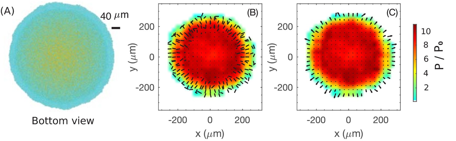
Coarse-grained view of director, velocity and pressure fields in the bottom layer of colony.

(A) The bottom view of a simulated colony. Color scheme is the same as in Figure 4A. (B) Bars show the planar component of the coarse-grained director field at the bottom layer. (C) Arrows show the planar component of the coarse-grained velocity field at the bottom layer. Colors in (B) and (C) indicate the local pressure; see scale bar on the far right. The pressure is expressed in unit of $P_{0} = γ_{s u r f} / w_{0}$ where $γ_{s u r f}$ is the surface tension, the main force underlying pressure build-up in our model.

https://doi.org/10.7554/eLife.41093.015

Figure 7

Download asset Open asset

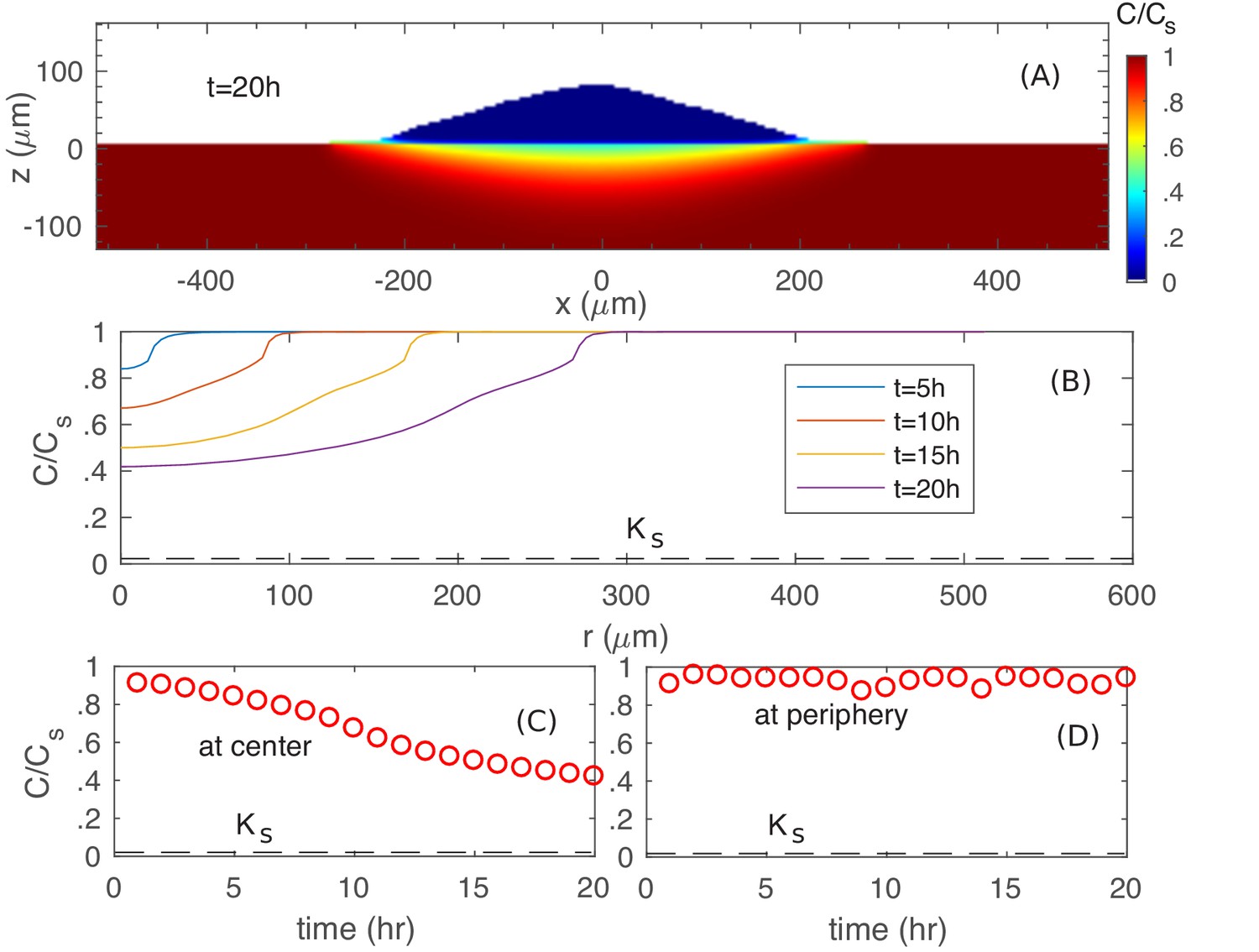
Spatiotemporal nutrient profiles.

(A) The xz cross sectional view of the nutrient concentration inside the colony and in the agar, at time $t = 20 h$ . (B) The nutrient profile at the agar surface for different times. The nutrient concentration vs. time at the center (C) and at the periphery (D) of the colony at the agar surface.

https://doi.org/10.7554/eLife.41093.016

Figure 8 with 2 supplements

Download asset Open asset

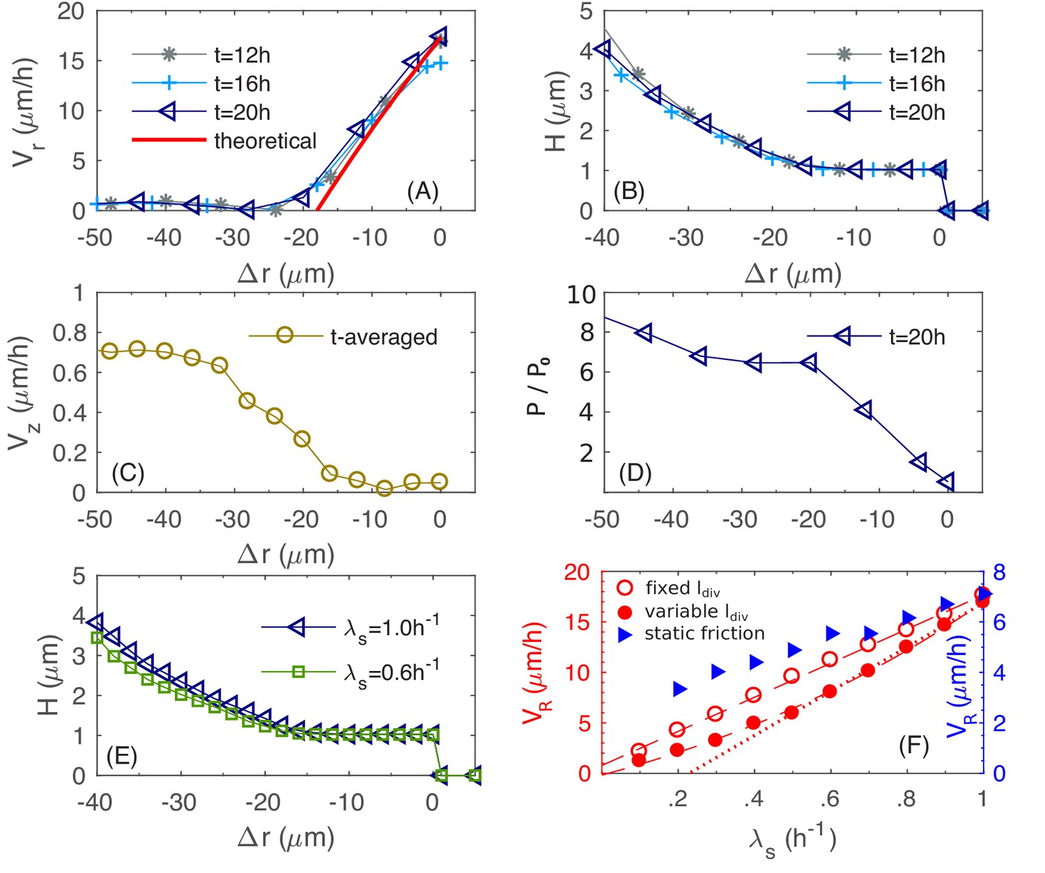
Physical characteristics near the outer periphery of the colony.

(A) The azimuthally averaged local speed of radial expansion $V_{r}$ vs. the signed distance $Δ r$ from the edge of the colony (cf. Equations (A1.5.1) in Appendix 1) at various times. (B) The azimuthally averaged local height $H$ vs. $Δ r$ at various times. (C) The azimuthally averaged local speed of vertical expansion $V_{z}$ vs. $Δ r$ , averaging over $t = 12, 16, 20$ hr. (D) The azimuthally averaged local pressure $P$ vs. $Δ r$ at time $t = 20 h .$ As in Figure 6, pressure is expressed in unit of $P_{0} = γ_{s u r f} / w_{0}$ . (E) The azimuthally averaged height $H$ vs. $Δ r$ at growth rate $λ_{S} = 0.5 h^{- 1}$ and $1.0 h^{- 1}$ . (F) The simulated colony horizontal expansion speed $V_{R}$ vs. the batch culture growth rate $λ_{S}$ with a fixed $l_{d i v}$ (red open circles) and a growth-rate dependent $l_{d i v}$ (red closed circles) using dynamic friction. The dashed line that fits the open circles is given by $V_{R} = 16.9 λ_{S} + 0.8$ ; the solid line that fits the closed circles for $λ_{S} \geq 0.5 h^{- 1}$ is $V_{R} = 5.7 λ_{S} l_{d i v} - 0.2$ ; the dash dotted line fits the closed circles with $V_{R} = 22.1 λ_{S} - 5.2$ . In these expressions, the speeds are in unit of $μ m/h$ and growth rate in $h^{- 1}$ . For comparison, we also include simulated $V_{R}$ vs. $λ_{S}$ with a growth-rate dependent $l_{d i v}$ , for a model with static friction alone (see Equations (A1.4.6) of Appendix 1) between cell and agar (blue triangles).

https://doi.org/10.7554/eLife.41093.017

Figure 8—figure supplement 1

Download asset Open asset

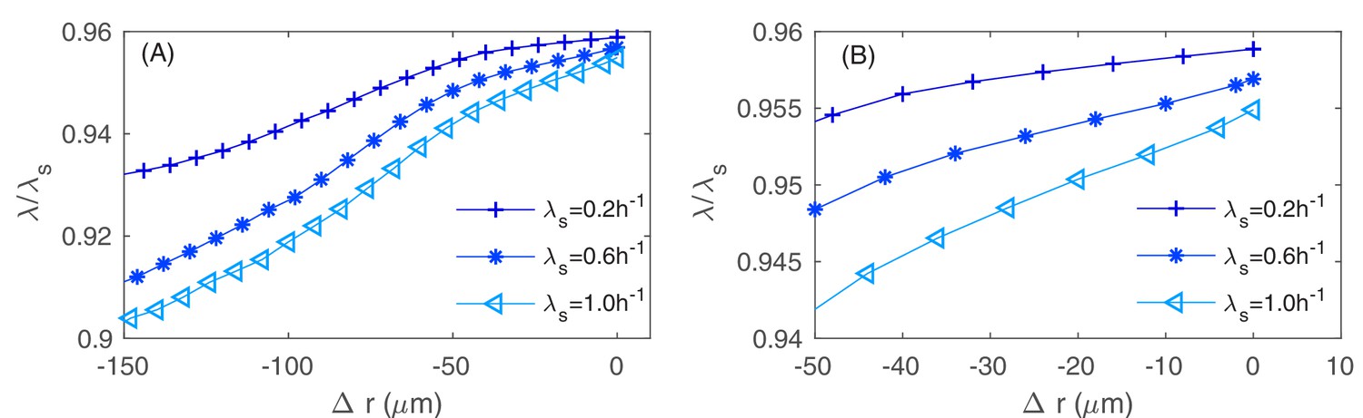
The azimuthally averaged and rescaled local growth rate $λ / λ_{S}$ as function of the signed distance $Δ r$ to the colony rim with various values of the batch culture growth rate $λ_{S}$ .

Precise definition of this signed distance $Δ r$ is given in Equations (A1.5.1) in Appendix 1.5 on coarse-grained variables. At the rim $Δ r = 0$ , the nutrient concentration $C$ is close to $C_{s}$ , the constant concentration value in the boundary condition, and $λ / λ_{S}$ is close to $C_{s} / (C_{s} + K_{S})$ , which is $0.96$ with our choice of parameters $C_{s} = 0.5 m M$ and $K_{S} = 0.02 m M$ . (A) The average is taken over the entire colony, where the variation of the (rescaled) local growth rate is within $6 %$ . (B) The average is taken over $1 / 3$ of the colony near the rim, where the variation of the (rescaled) local growth rate is within $2 %$ .

https://doi.org/10.7554/eLife.41093.018

Figure 8—figure supplement 2

Download asset Open asset

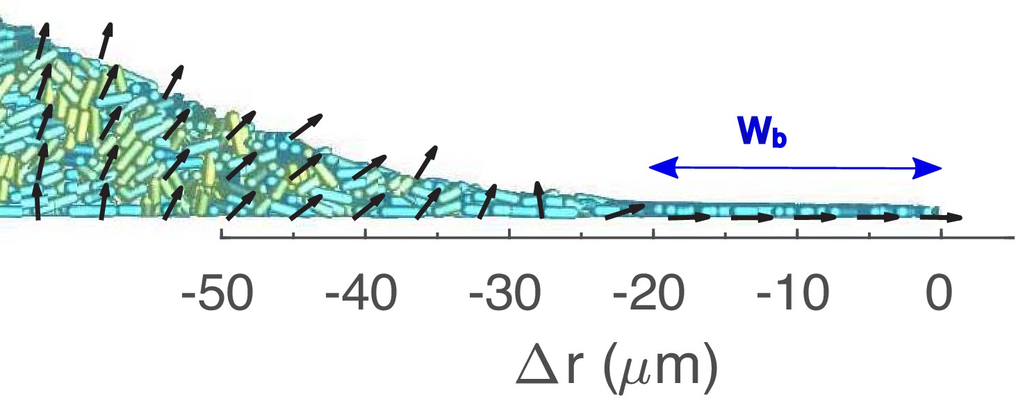
A zoomed in view of the periphery of the colony shown in Figure 4A, overlaid with coarse-grained velocity field (zoomed in view of the same periphery region in Figure 4D).

$Δ r$ is the signed distance from the edge of the colony. $W_{b}$ is the buckling width.

https://doi.org/10.7554/eLife.41093.019

Figure 9

Download asset Open asset

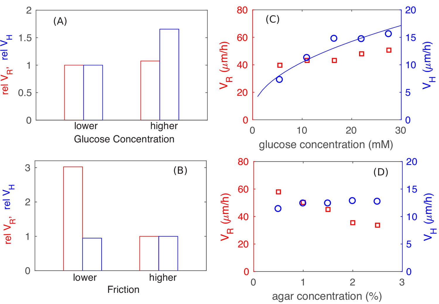
Parameter dependence of colony growth characteristics.

Simulation results using the full model with 2x increase in glucose concentration (panel A) and 4x decrease in all frictional parameters (panel B) for $V_{R}$ (red bars) and $V_{H}$ (blue bars). Specifically, in panel (A) we fix the friction at a high level (with $μ_{c a} = 0.8, μ_{c c} = 0.1, γ_{c c, t} = 10000 μ m^{- 1} h^{- 1}$ , and $h_{r a n} = 0.1 μ m$ ), and use $C_{s} = 0.5 m M$ as the lower glucose concentration, $C_{s} = 1.0 m M$ as the higher glucose concentration. In panel (B), we fix the glucose concentration at the lower level ( $C_{s} = 0.5 m M$ ), and vary the friction, from the higher value of $μ_{c a} = 0.8, μ_{c c} = 0.1, γ_{c c, t} = 10000 μ m^{- 1} h^{- 1}$ , $h_{r a n} = 0.1 μ m$ used in (A) to the lower value of $μ_{c a} = 0.2, μ_{c c} = 0.025, γ_{c c, t} = 2500 μ m^{- 1} h^{- 1}$ , $h_{r a n} = 0.025 μ m$ . The corresponding experimental results are shown in panels C and D: In (C), glucose concentration was varied with agar density fixed at 1.5%. In (D), agar density was varied with glucose fixed at 0.2% (w/v). The data for $V_{H}$ in panel C is consistent with a square root dependence on nutrient concentration (blue line) expected from the basic analysis in Figure 5.

https://doi.org/10.7554/eLife.41093.020

Figure 9—source data 1 Experimental data on the horizontal and vertical colony expansion speeds at various glucose and agar concentrations.: https://doi.org/10.7554/eLife.41093.021
Download elife-41093-fig9-data1-v1.xlsx

Figure 10

Download asset Open asset

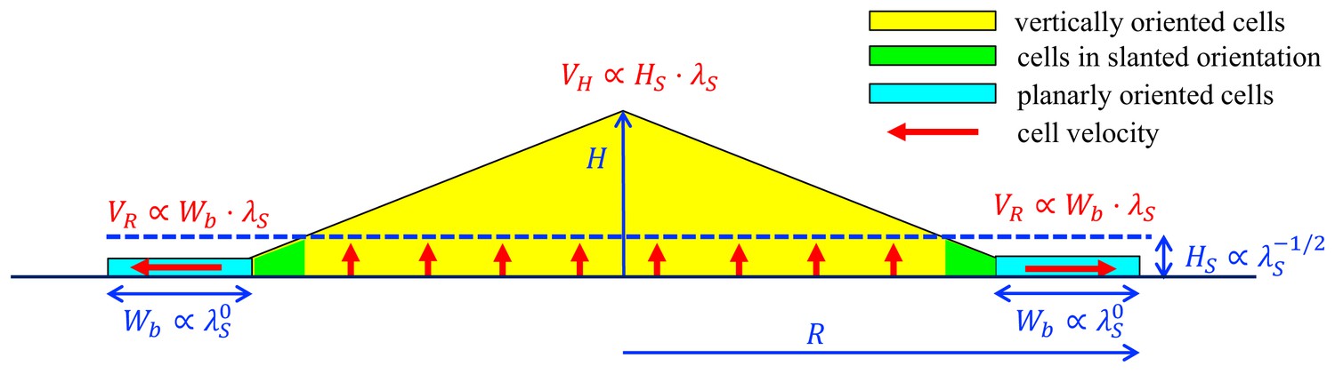
A schematic summary of key mechanisms in the growth of an E.coli colony.

After an initial, exponential monolayer growth, buckling occurs at the center of the colony. Cells then grow actively only in the bottom layers (red vertical arrows) whose thickness ( $H_{S}$ ) is determined by the nutrient penetration level (dashed blue line). Cells lying above them are passively pushed up. Throughout this yellow triangular region, cells are oriented vertically. Near the colony edge (cyan region), the cells are oriented planarly and grow outward (horizontal red arrow) continuously in a spread mode to expand the colony in the radial direction. The width of this annulus ( $W_{b}$ ) is determined by mechanical effects arising from the surface tension which pulls the thin layer of cells into the agar, and cell-agar friction which builds up the pressure from the outer edge of the layer, eventually causing buckling at an inner radius where cells transition to the vertical orientation (the green region). These two characteristic parameters, $H_{S}$ and $W_{b}$ , set the speeds of radial and vertical expansions, $V_{R}$ and $V_{H}$ , respectively, as shown in red. The growth rate dependence of these parameters is shown in blue.

https://doi.org/10.7554/eLife.41093.022

Figure 11

Download asset Open asset

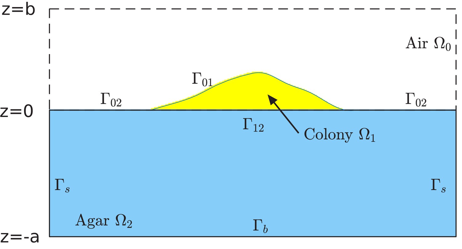
Schematic of the computational box and different regions in the model of simulation.

The computational box is $Ω = (- L, L) \times (- L, L) \times (- a, b)$ , where all $L$ , $a$ , and $b$ are positive numbers in the units of length. This box is divided into the air region $Ω_{0}$ , colony region $Ω_{1}$ , and agar region $Ω_{2} = (- L, L) \times (- L, L) \times (- a, 0)$ , respectively. See Supplementary file 1-Table S5 for typical values of $L$ , $a$ , and $b$ used in our simulations. The colony surface or colony-air interface $Γ_{01}$ separates the colony from air. The plane $z = 0$ in the computational box is divided into two parts. One is the interface that separates the colony from agar, and is denoted by $Γ_{12}$ . The remaining part, denoted $Γ_{02}$ , separates the air from agar. Note that, since the bacterial colony grows with time $t$ , all the air region $Ω_{0}$ , the colony region $Ω_{1}$ , the colony-air interface $Γ_{01}$ , and the colony-agar interface $Γ_{02}$ depend on time $t$ .

https://doi.org/10.7554/eLife.41093.023

Figure 12

Download asset Open asset

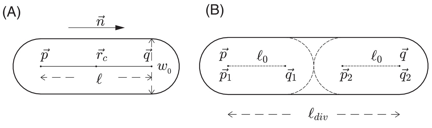
Schematic view of cell growth and division.

(A) A sphero-cylinder model of an E.coli cell. Here, $w_{0}$ is the diameter of each of the hemispheres, $\vec{p}$ and $\vec{q}$ are the centers of these hemispheres, $l = | \vec{p} - \vec{q} |$ is the cylindrical length of the cell, $\vec{n} = (\vec{p} - \vec{q}) / l$ is the unit vector along the cylindrical axis of the cell, and ${\vec{r}}_{c}$ is the center of the cell. (B) Cell division. Once the cylindrical length of a cell reaches a critical value $l_{d i v}$ , the cell divides into two daughter cells. The two centers of hemispheres of the mother cell become the centers of hemispheres of the daughter cells. Each of these two daughter cells has the cylindrical length $l_{0}$ with fluctuations, where $l_{0}$ is a constant cylindrical length for any new born cell and any initial cell in the simulation. Fluctuations of angular velocities are also introduced for the daughter cells; cf. Appendix 1.3.

https://doi.org/10.7554/eLife.41093.024

Figure 13

Download asset Open asset

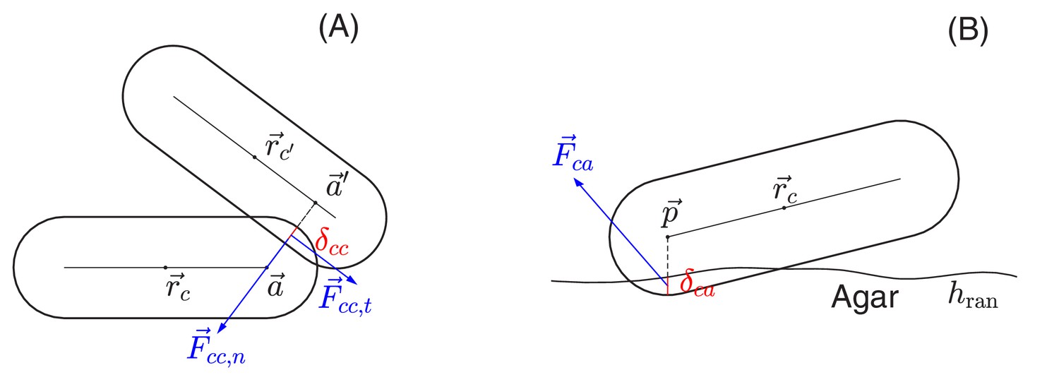
Schematic view of cell-cell and cell-agar interactions.

(A) Cell-cell interaction. Two cells, centered at ${\vec{r}}_{c}$ and ${\vec{r}}_{c^{'}}$ , respectively, are in contact with each other. The shortest distance between the central cylindrical lines of the two cells is $d = |\vec{a} - {\vec{a}}^{'}|$ with $\vec{a}$ and ${\vec{a}}^{'}$ two points on the cylindrical central lines of these two cells, respectively. The amount of the overlap of these two cells is $δ_{c c} = w_{0} - d$ . We shall denote by ${\vec{r}}_{c c}$ the center of the line segment connecting $\vec{a}$ and ${\vec{a}}^{'} .$ The total interaction force, exerted at center ${\vec{r}}_{c c}$ , is the sum of the normal force ${\vec{F}}_{c c, n}$ in the normal direction ${\vec{n}}_{c c} = (\vec{a} - {\vec{a}}^{'}) / d$ and the tangential force ${\vec{F}}_{c c, t}$ in a direction orthogonal to ${\vec{n}}_{c c}$ that is determined by the relative velocities of these two cells; see the details in Appendix 1.4 on force calculations. (B) Cell-agar interaction. A cell, centered at ${\vec{r}}_{c}$ , touches the agar surface that has the mean position at $z = 0$ and the roughness $h_{r a n}$ (the maximum fluctuation around the mean), with $δ_{c a}$ the amount of the overlap of the cell and agar. If the center of the hemispherical cap of the cell corresponding to the end that dips into the agar is $\vec{p} = (x_{a}, y_{a}, z_{a})$ , then $δ_{c a} = w_{0} / 2 - z_{a}$ . Denote ${\vec{r}}_{c a} = (x_{a}, y_{a}, z_{a} - w_{0} / 2)$ , which is the midpoint of the line segment along the vertical line passing through the point $\vec{p}$ between $z = 0$ and $z = - δ_{c a}$ . The total cell-agar interaction force ${\vec{F}}_{c a}$ , exerted at the center ${\vec{r}}_{c a}$ , is the superposition of a normal force ${\vec{F}}_{c a, n}$ in the vertical direction and the tangential force ${\vec{F}}_{c a, t}$ in a direction along the $x y$ plane that is determined by the velocity of the cell; cf. Appendix 1.4.

https://doi.org/10.7554/eLife.41093.025

Figure 14

Download asset Open asset

Schematic view of surface tension acting on cells at the colony boundary.

(A) a snapshot of part of a growing colony from a typical computer simulation. The red curve defines the macroscopic colony-air interface which is used in updating the nutrient profile; cf. $Γ_{01}$ in Figure 11 and Appendix 1.1. Cells on the top of the colony are held down by the surface tension force. (B) A sequence of configurations of colony during the early stage of growth. Top: Initial cells grow exponentially and form a monolayer. All cells in this layer are held down by the surface tension force. Middle: As more cells are born in the monolayer, the frictions between these cells and the rough agar surface increase. The competition between such frictions and the surface tension force that pulls down cells leads to an accumulation of the lateral pressure in the cells. The monolayer buckles up once that the surface tension can no longer hold down all the cells in the monolayer. Such buckling occurs at certain radial distance from the center of colony; cf. Figure 8D. Bottom: Once the monolayer buckles, the colony starts to grow vertically. In the meantime, the buckling region moves outward as the colony expands radially. (C) The parameters used in the definition of surface tension force. The parameter $h_{c e l l}$ is the height of a cell that sticks out of the macroscopic colony surface; it is measured from the mean height of the agar surface $z = 0$ to the 'tallest point' in the cell. The blue and red lines describe the macroscopic water level (indicated by $h_{w}$ ) and colony height (indicated by $h$ ), respectively. The parameter $δ_{h}$ is used to control how tightly the surface tension holds back those cells on the top of the colony. See more details in Appendix 1.4c.

https://doi.org/10.7554/eLife.41093.026

Appendix 1—figure 1

Download asset Open asset

Schematic view of a nested finite difference grid for the agar region $Ω_{2}$ .
https://doi.org/10.7554/eLife.41093.029

Appendix 1—figure 2

Download asset Open asset

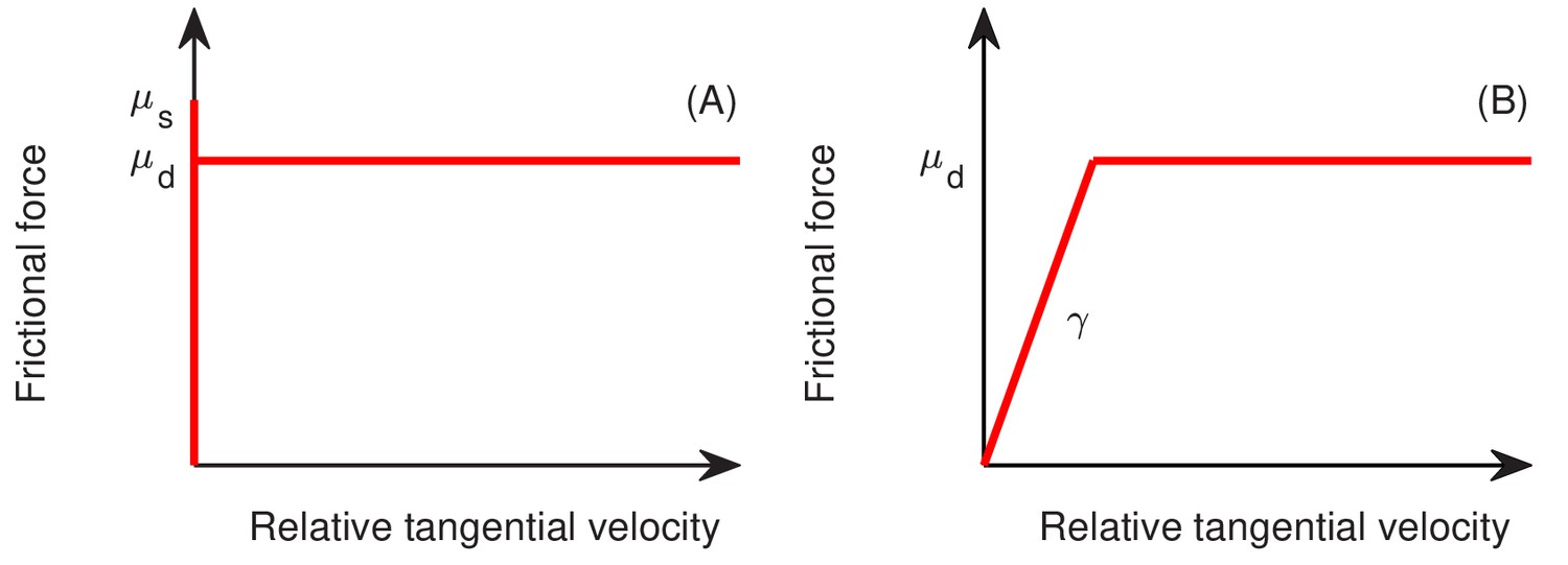
The standard (A) and modified (B) model for friction between two objects, as a function of tangential relative velocity between the two objects, where $μ_{s}$ and $μ_{d}$ are the static and dynamic friction constants, respectively.
https://doi.org/10.7554/eLife.41093.030

Appendix 1—figure 3

Download asset Open asset

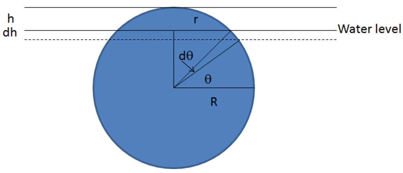
Schematic of the derivation of the surface tension force.
https://doi.org/10.7554/eLife.41093.031

Appendix 2—figure 1

Download asset Open asset

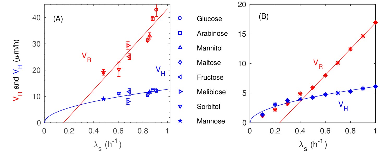
Experimental measurement on $V_{R}$ and $V_{H}$ with various batch culture growth rates.

Data are fitted with the stright line $V_{R} = 51.27 λ_{S} - 7.96$ and the squre root curve $V_{H} = 12.7 \sqrt{λ_{S}}$ for the redial and vertical speeds of expansion $V_{R}$ and $V_{H}$ respectively. (B) Simulation results on $V_{R}$ and $V_{H}$ with various batch culture growth rates and with a variable diviting length $l_{d i v}$ . data are fitted for $λ_{S} \geq 0.5 h^{- 1}$ using the straight line $V_{R} = 22.1 λ_{S} - 5.24$ the squre-root curve $V_{H} = 6.12 \sqrt{λ_{S}},$ respectively.

https://doi.org/10.7554/eLife.41093.033

Appendix 2—figure 2

Download asset Open asset

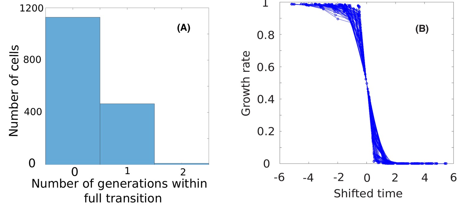
Statistics of cells undergoing growth transition.

(A) The histogram of the number of generations of the cells that experienced high-to-low growth rate transition.(B) Curves of growth rates vs. shifted time for 100 cells randomly selected from those 80% cells.

https://doi.org/10.7554/eLife.41093.034

Author response image 1

Download asset Open asset

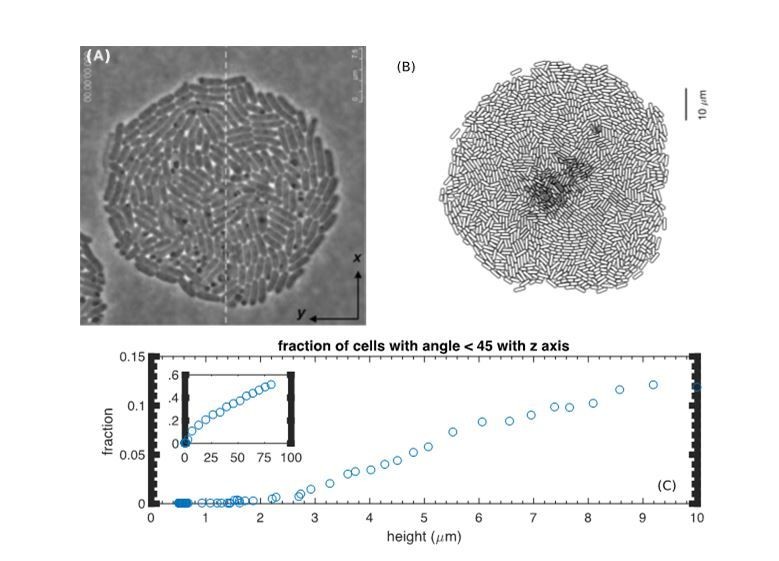
Lack of verticalization for thin colonies.

(A) Reproduction of Figure 2A from (Su et al., 2012). (B) Bottom view of a simulated colony at t=7h. (C) The fraction of vertically oriented cells (defined by the angle with the z-axis less than 45 degrees) vs. height from the simulation.

https://doi.org/10.7554/eLife.41093.036

Author response image 2

Download asset Open asset

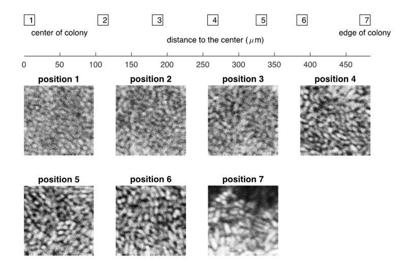
Experimental results on the confocal images of a bacterial colony at different positions, from the center to the edge.

The bacterial strain and the growth medium are the same as described in “Experimental Methods” in the main text, except that the thickness of agar dish is ~0.3mm. The picture was taken at roughly 24 hours after the initial inoculation.

https://doi.org/10.7554/eLife.41093.037

Author response image 3

Download asset Open asset

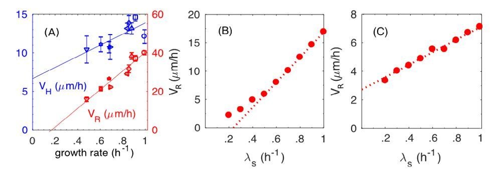
The dynamic and static friction models distinguished by the growth-rate dependence of radial expansion speed.

(A) From main text Figure 1F. Experimental results on the radial speed VR and the vertical speed VH with respect to various batch culture growth rates. (B) From Figure 8F in the main text (new version). Simulation results of radial speed VR of the colony, where both static and dynamic frictions are included in simulations. (C) New simulation results of radial speed VR of the colony, where only the static friction is included.

https://doi.org/10.7554/eLife.41093.038

Additional files

Supplementary file 1 Supplemental tables S1-5.: https://doi.org/10.7554/eLife.41093.027
Download elife-41093-supp1-v1.pdf

Download links

A two-part list of links to download the article, or parts of the article, in various formats.

Downloads (link to download the article as PDF)

Open citations (links to open the citations from this article in various online reference manager services)

Mendeley

Cite this article (links to download the citations from this article in formats compatible with various reference manager tools)

Mya R Warren
Hui Sun
Yue Yan
Jonas Cremer
Bo Li
Terence Hwa

(2019)

Spatiotemporal establishment of dense bacterial colonies growing on hard agar

eLife 8:e41093.

https://doi.org/10.7554/eLife.41093

Sign up for email alerts

Privacy notice