Statistical structure of locomotion and its modulation by odors
- Duke University, United States
Figures
Figure 1 with 1 supplement
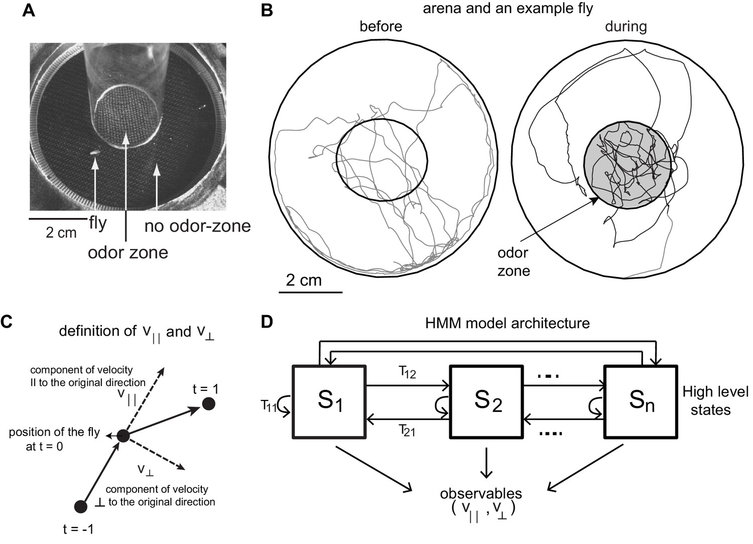
Experimental setup and HMM architecture.
(A) Top view of the chamber. (B) Tracks of an example fly in a circular arena (3.2 cm in radius). The central region (1.2 cm radius) has no odor during the first 3 min (before period) and is odorized in the last 3 min (during odor). The odor zone is shaded. (C) The observables - and at time point t = 0 are schematized. is the component of the fly’s velocity along the velocity vector at the previous time point; is the component perpendicular to the velocity vector at the previous time point. (D). HMM Model Architecture: A single layered model with n states each defined by a joint probablity distribution of the observables. The probability of transitioning from the ith state to the jth state is given by Tij.
Figure 1—figure supplement 1
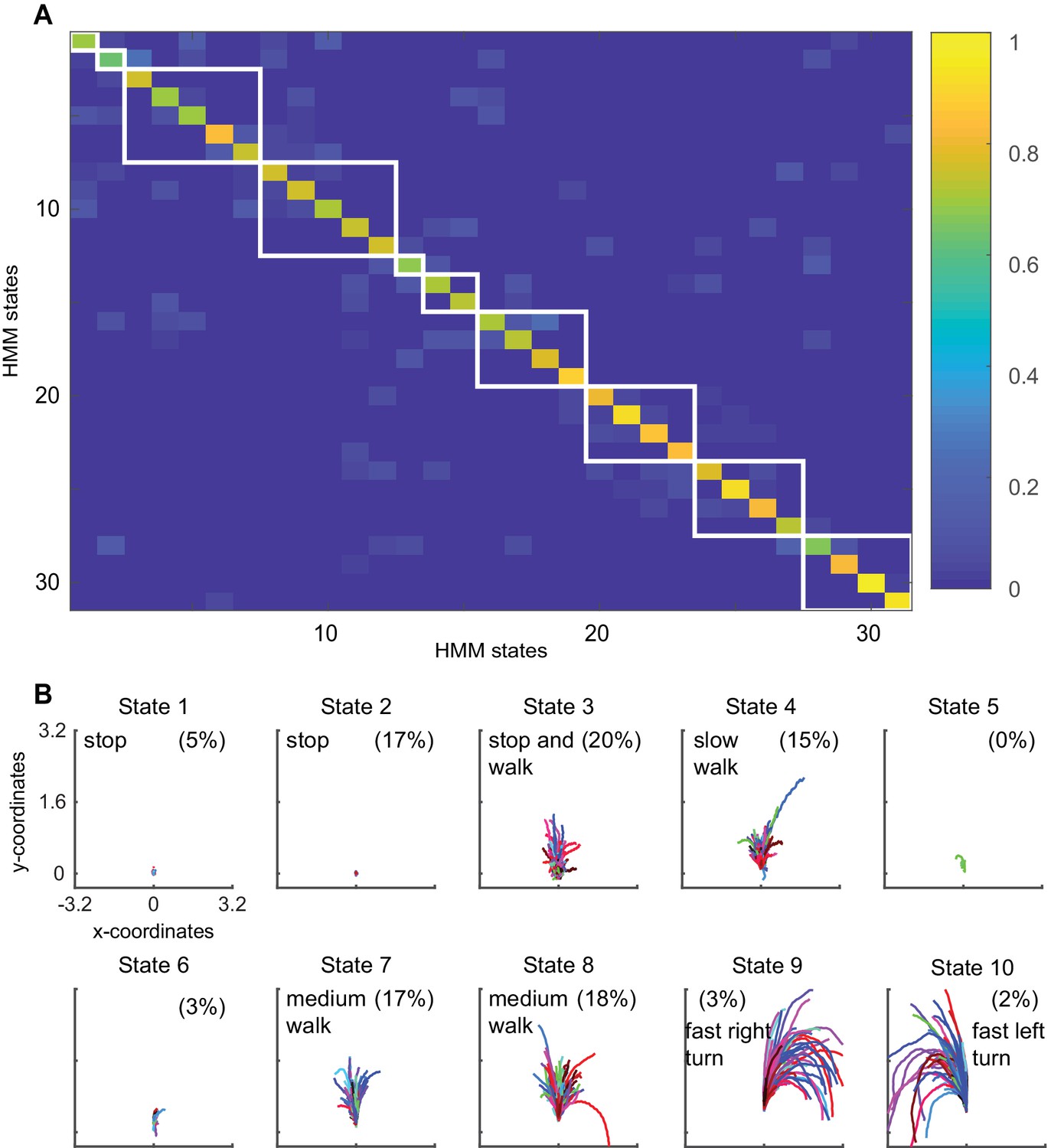
Block clustering of HMM states suggests a small number of locomotor features.
(A) Transition probability matrix of the 31 used HMM states. The states are block clustered based on the probability of transitioning to the other states. White boxes are drawn around states that were clustered together. Clustered states were sorted in the ascending order of mean speed/standard deviation of curvature, with state 1 being low-speed-high-curvature and state 10 being high speed and low curvature. (B) Forward trajectories of the resultant clusters. States 1 through 10 correspond to the white boxes in A as shown in order from top left to bottom right.
Figure 2 with 3 supplements
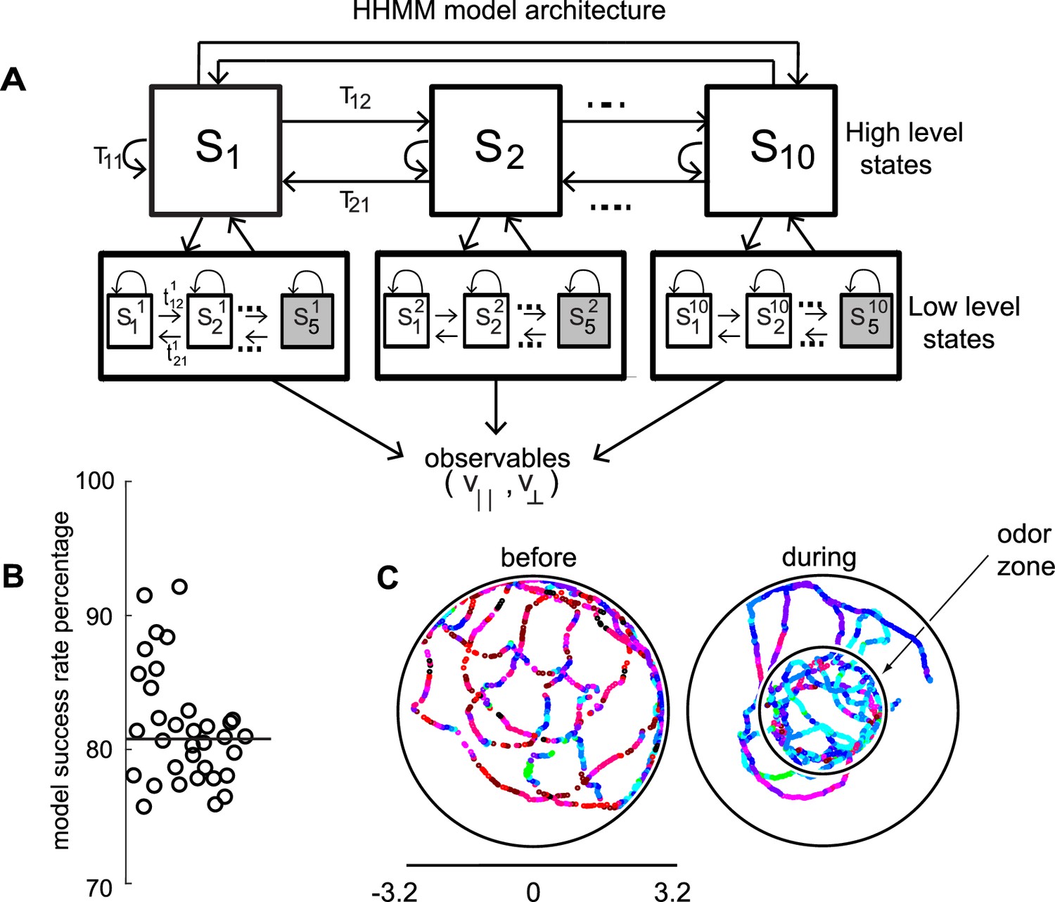
HHMM architecture.
(A) Model architecture: The model consists of two layers; there are 10 high level states (HL states) each of which have five low level (LL) states. The probability of transitioning from the ith HL state to the jth HL state is given by Tij. At the lower level, each HL state has its own transition probability matrix that describes transitions between its LL states. The shaded boxes represent the terminal states. (B) As a measure of the model’s ability to fit the data for individual flies in our dataset - the percentage of timepoints for which the model had >85% confidence is plotted. Black line is the median. (C) HL state assignment for a single fly. The 10 high level states, each coded using a different color are overlayed on the tracks of a fly.
Figure 2—figure supplement 1
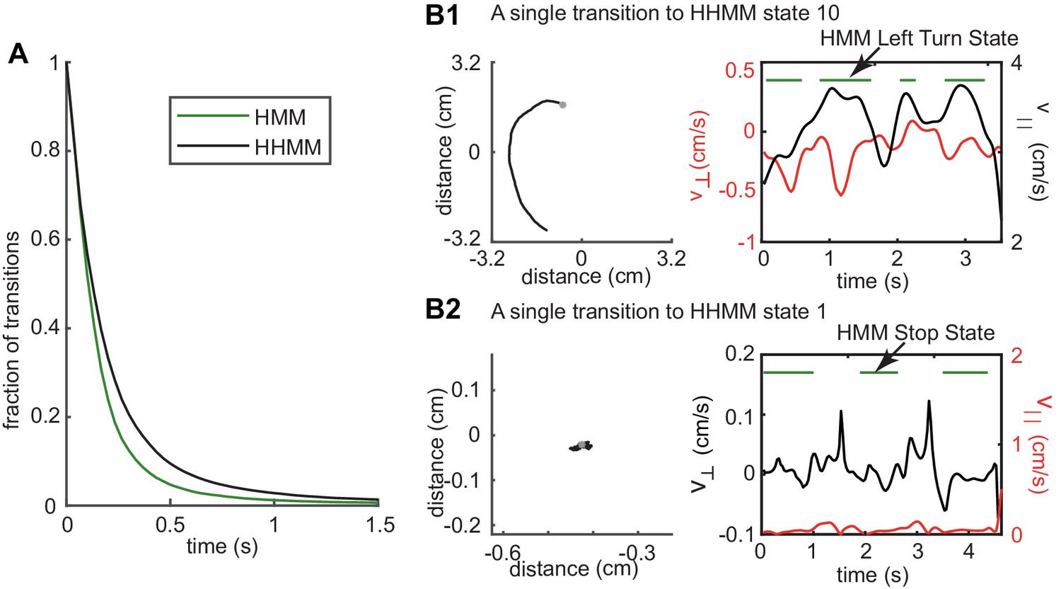
Longer duration of HHMM states allows it to discover structure in the data over longer times.
(A) Complementary cumulative distribution (cCDF) of tracks for HHMM vs. HMM states showing that HHMM states have many more tracks with longer durations. (B1) An example track that represents a single HHMM state. HMM detects this track as a left turn but its assignment of the track as a left turn (green lines) is intermittent. (B2) Another example - in this case for a stop state. In both examples, changes in the value of the observables result in the intermittency of the HMM state. The observable resulting in the intermittency is colored red. In the case of B1, small straight segments within the left turn result in the intermittency. In the case of B2, small movements cause an exit from the stop state.
Figure 2—figure supplement 2
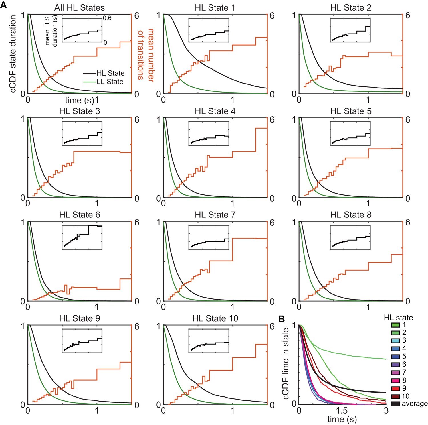
HL states have a longer duration than LL states because of multiple transitions among low-level states/transition between HL states.
(A) Complementary cumulative distribution (cCDF) of durations for HHMM HL states (black) and the corresponding LL states (green). Mean number of LL state transitions per HL state transition increases with the duration of the HL state (orange). Inset black line shows the mean duration of LL states for each HL state track. (B) cCDF of the total time spent in a state of a given duration.
Figure 2—figure supplement 3
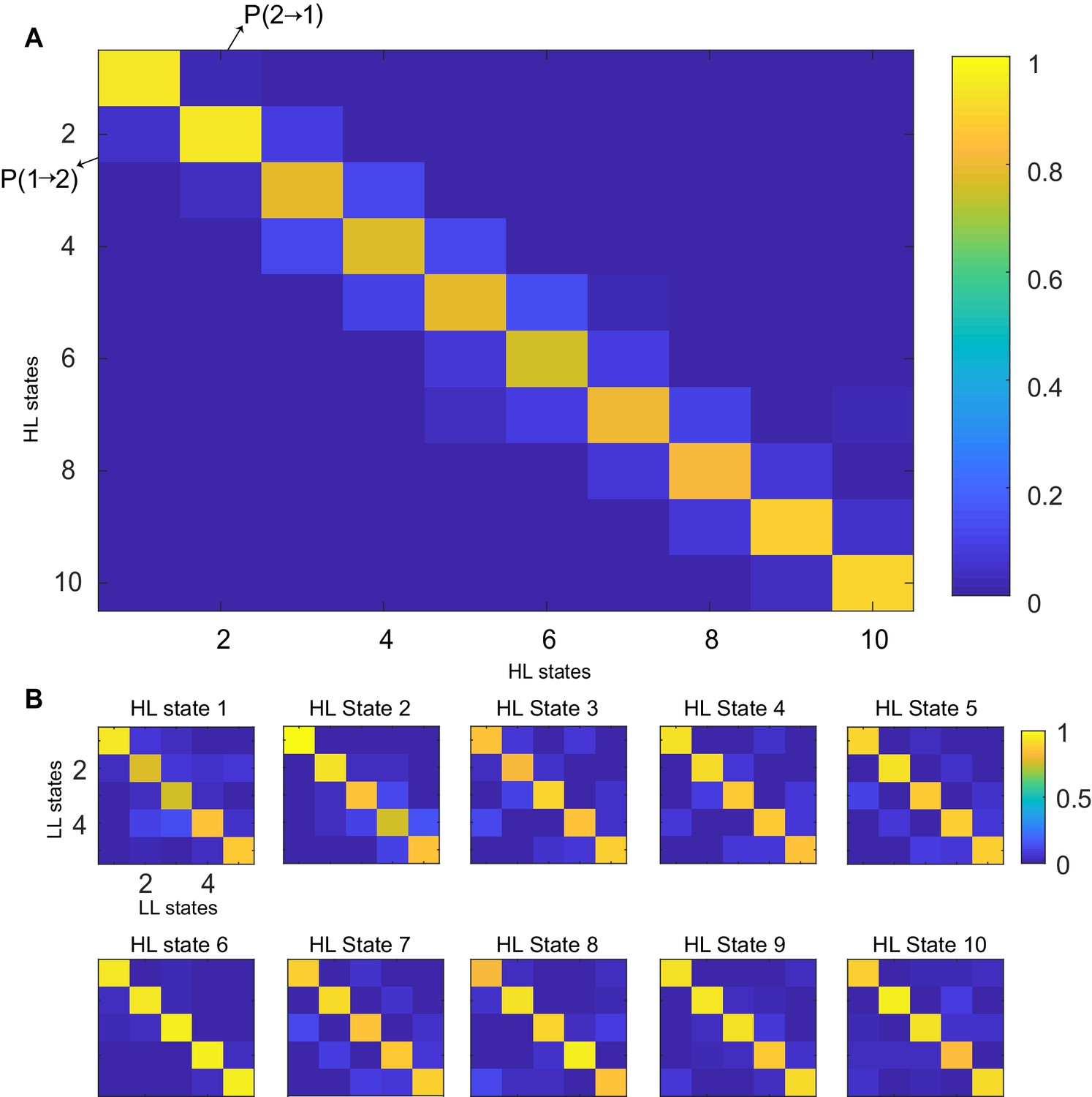
Transition probability matrices.
(A) Transition probability matrix for HL states. States were sorted in the ascending order of average speed/standard deviation of curvature, with state 1 being low-speed-high-curvature and state 10 being high speed and low curvature. (B) Transition matrices of LL states for every HL state. Each HL state has five LL states.
Figure 3 with 1 supplement
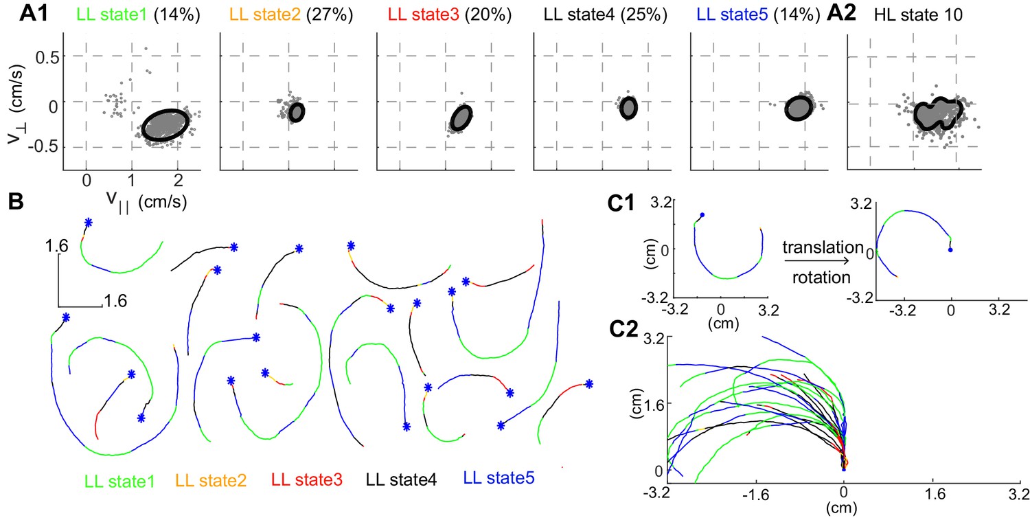
Structure of a HL state.
(A1) 85% confidence bounds of the model (black ellipse) and a random sample of observables (gray dots) corresponding to data points assigned to the LL states underlying HL state 10. Percentage of time spent in a given LL state is also shown. (A2) Distribution of observables for the HL state. (B) Example tracks denoting a single transition to HL state 10 show that the fly is turning counterclockwise. LL states were color coded. (C1) Each track is rotated and translated for visualization. (C2) All 20 tracks in B were transformed as shown in C1. Transformation reveals that all HL state 10 trajectories represent left turns.
Figure 3—figure supplement 1
LL states corresponding to each HL statest: The same plot as Figure 3A for all the states.
State 10's distribution has been replicated for completeness.
Figure 4
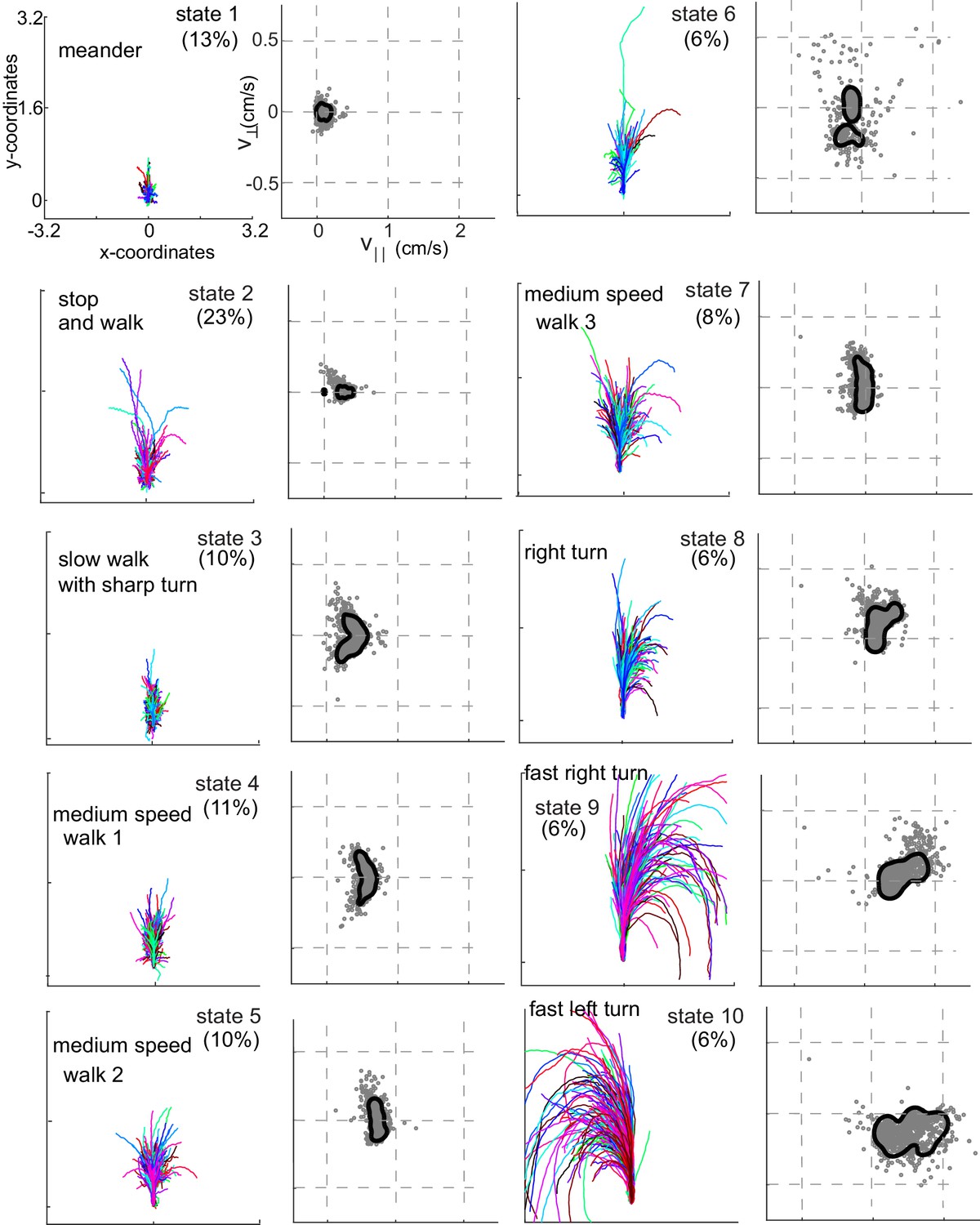
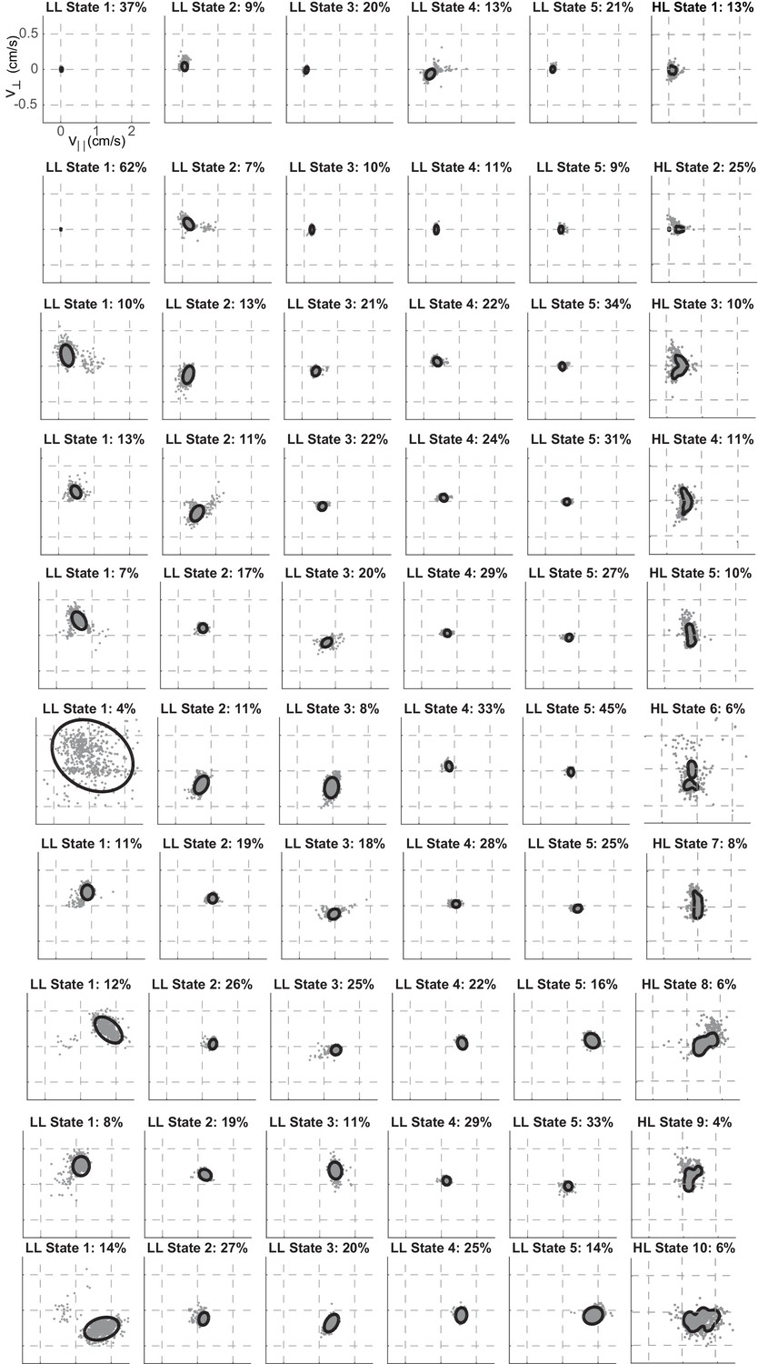
Each HL state describes a locomotor feature during which the fly uses a narrow region of the velocity space.
Trajectories (left) and distribution of observables (right) corresponding to each of the 10 HL states are shown. Trajectories were transformed via translation and rotation to start at the origin, and the initial velocity vector pointed along the y-axis. Both model distribution (solid lines) and randomly selected 1000 empirical datapoints (gray dots) belonging to a given state are shown. The percentage of time a fly spends in a given HL state is shown.
Figure 5 with 1 supplement

Odors modulate locomotion by altering the time spent in different HL states.
(A) Odor-induced changes in the occupancy of HL states inside the odor-zone. Bar graphs showing the probability distribution of the 10 HL states during odor, before odor, the difference between the two and the fractional change in the distributions when the fly is inside. Red lines show ±bootstrapped 95% confidence intervals. Asterisks indicate significance at 0.05 with Bonferroni-Holm correction (**) and 0.01 (*) without correction based on bootstrapped hypothesis testing for equality of means. (B) Same as in A, but for outside the odor-zone.
Figure 5—figure supplement 1
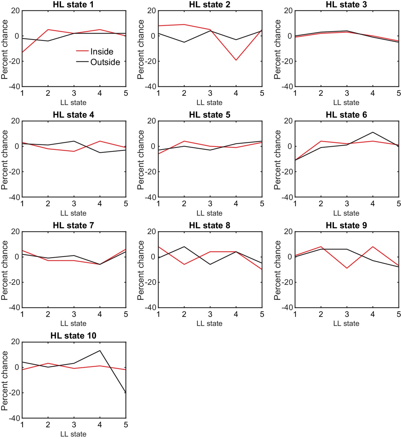
For each HL state, the composition of LL states remain the same .
Percent change before and during the presence of odor were calculated for inside and outside separately. No state occupancy changes by more than 20%.
Figure 6 with 1 supplement
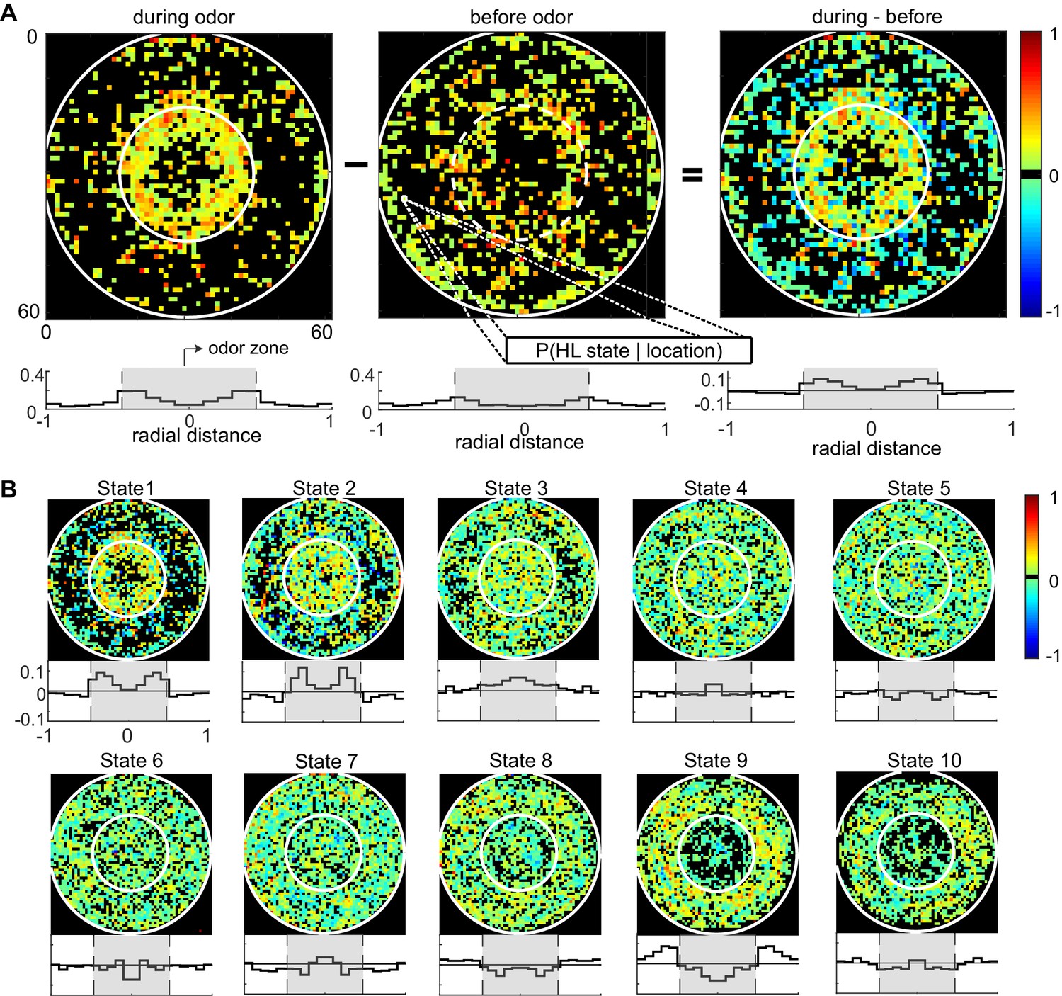
Fine spatial structure underlying odor-evoked changes in HL state occupancy.
(A) The probability distribution of HL states before and during odor was calculated for each of the 60 × 60 bins. Taking HL state 1 as an example, each specific bin represents the probability of HL state 1 given the spatial location. White circles show the extent of the odor-zone and the arena. Bottom row: Probability of HL state 1 as a function of radial distance. The shaded region indicates the odor zone. (B) Change in HL state occupancy for each of the 10 HL states.
Figure 6—figure supplement 1
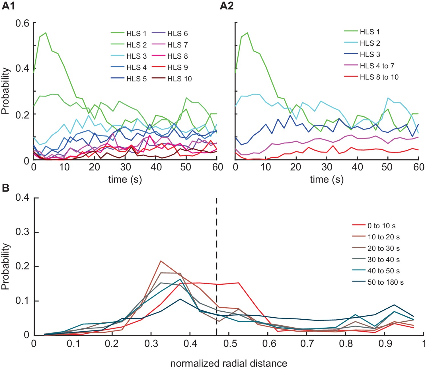
Temporal structure underlying HL state occupancy in response to odor.
(A1) Probability of HL state occupancy following first entry inside the peripheral odor zone (radius = 1.9 cm). (A2) Medium speed walking states (4-7) were grouped and high-speed turning states (8-10) were grouped together, and the mean HL state occupancy were calculated for the respective groups. (B) The radial occupancy of the flies at different time groups following first entry. The black vertical dotted line indicates the nominal odor boundary (radius = 1.5 cm).
Figure 7 with 5 supplements
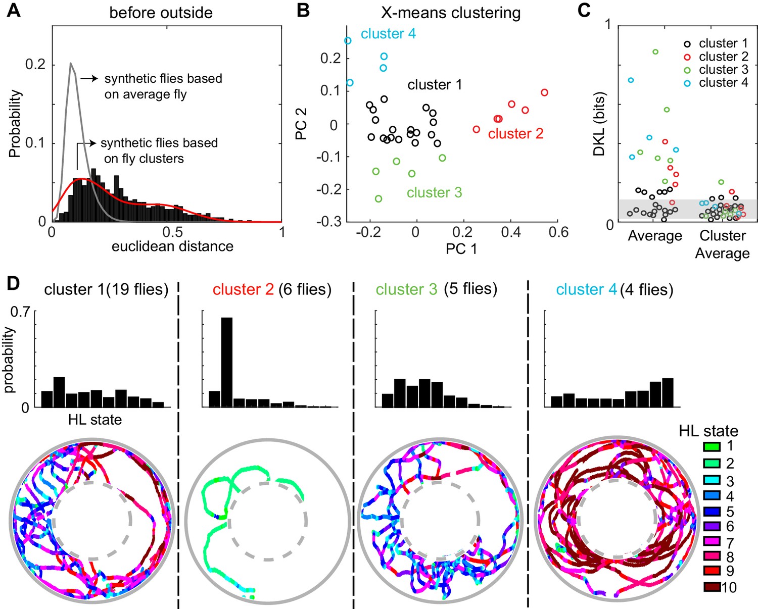
A fly’s locomotion cannot be explained as variations around an average fly and is well-described on the basis of three to four locomotor types.
(A) Histogram of distances between flies in the 10-dimensional space formed by the HL states. The distance between 100 iterations of 34 synthetic flies based on the average distribution of states is much smaller (gray line, Wilcoxon rank sum test, p < 10−131). The distance between synthetic flies drawn from four clusters of flies (red line) has a distribution more similar to the empirical distribution. (B) X-means clustering (a variant of K-means) in the 10-dimensional HL state space. Only the first two PCs are shown. Each cluster is represented by a different color. (C) Left: KL divergence from the average fly to the individual fly (n = 34). Right: KL divergence from the average fly in each cluster to each individual fly in the corresponding cluster. Shaded area reflects the expected KL divergence (99% of KL divergences) from the HL state distribution of the average fly to the HL distribution of synthetic flies generated from this average (n = 3400). (D) Average HL state distribution for each cluster is shown in the top row. Bottom row shows an example fly for each cluster with HL states overlayed.
Figure 7—figure supplement 1
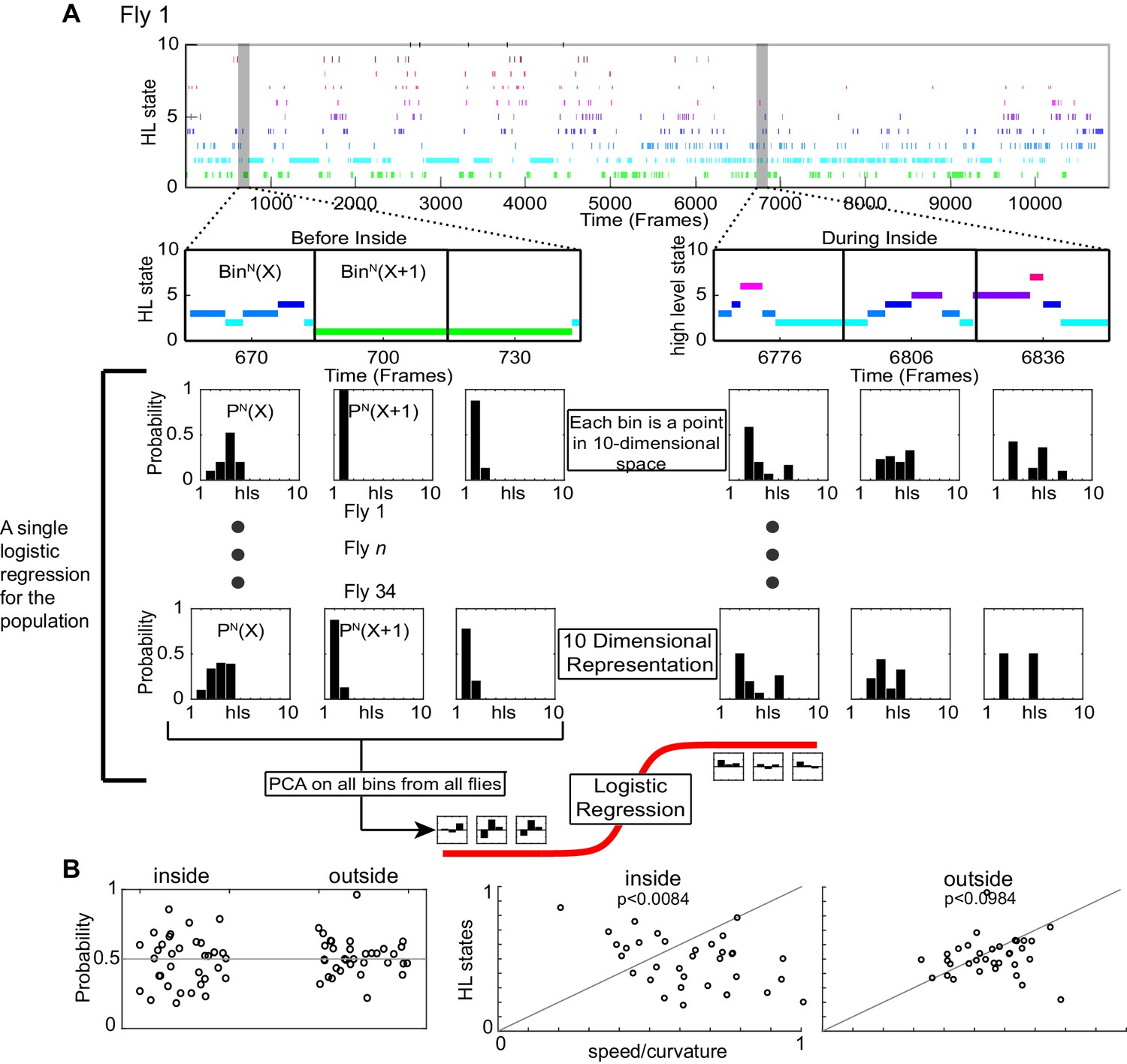
HL state distributions of the population are poor predictors for the presence of odor.
We used logistic regression to evaluate whether the distribution of HL states is predictive of the presence of odor. We know from Figure 6 that ACV causes a change in the distribution of HL states, and that these changes are different inside and outside the odor-zone. Therefore, we asked whether given that fly is either inside or outside the odor-zone, can we predict based on the distribution of HL states whether the fly is experiencing an odor. (A) An example of HL state as a function of time for a single fly. The HL states were segmented into 1 second chunks and further subdivided into each of the four scenario - before inside, during inside, before outside and during outside. Only the before inside and during inside cases are shown. The HL state distributions were calculated for each segment. Thus, each 1 second bin is represented as a point in 10-dimensional state. The process was repeated for each fly, PCA was performed on the entire dataset and only the principal components that explain >90% variance in the data were used to fit to a logistic regression (logit) model. (B) (Left) Results of a logarithmic regression (logit) model fit to the HL state distributions in 1 second segments for all flies do not show better probability of correct predictions over chance (gray line). (Right) Distributions of HL states of the population do not improve decoding over observables. (Wilcoxon signed rank test, p < 0.0084 for inside and p < 0.0984 for outside).
Figure 7—figure supplement 2
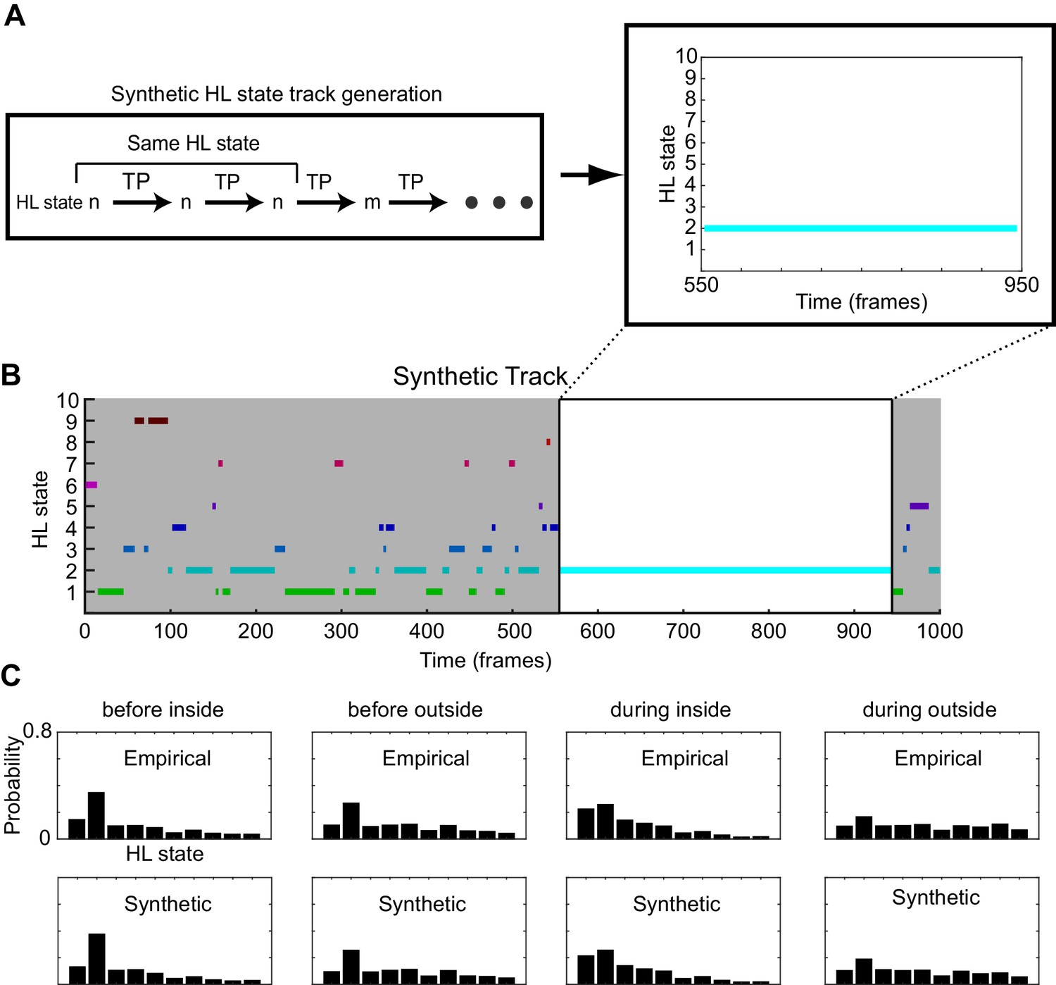
The process for generation of synthetic HL state sequences.
(A) A HL-state is sampled from the empirical average HL state distribution for a given scenario. Progression of HL states are calculated at each timepoint using the global transition probability matrices associated with the HHMM and the given scenario. Because of high probability of self-transitions, the HL state change only occurs after a few frames. A fragment is shown where a synthetic fly stays in HL state 2 for 400 frames. (B) A sample synthetic track. A synthetic track lasts for the median empirical duration of the given scenario (1000 frames are shown). (C) The mean empirical HL state distributions are similar to the mean synthetic HL state distributions.
Figure 7—figure supplement 3
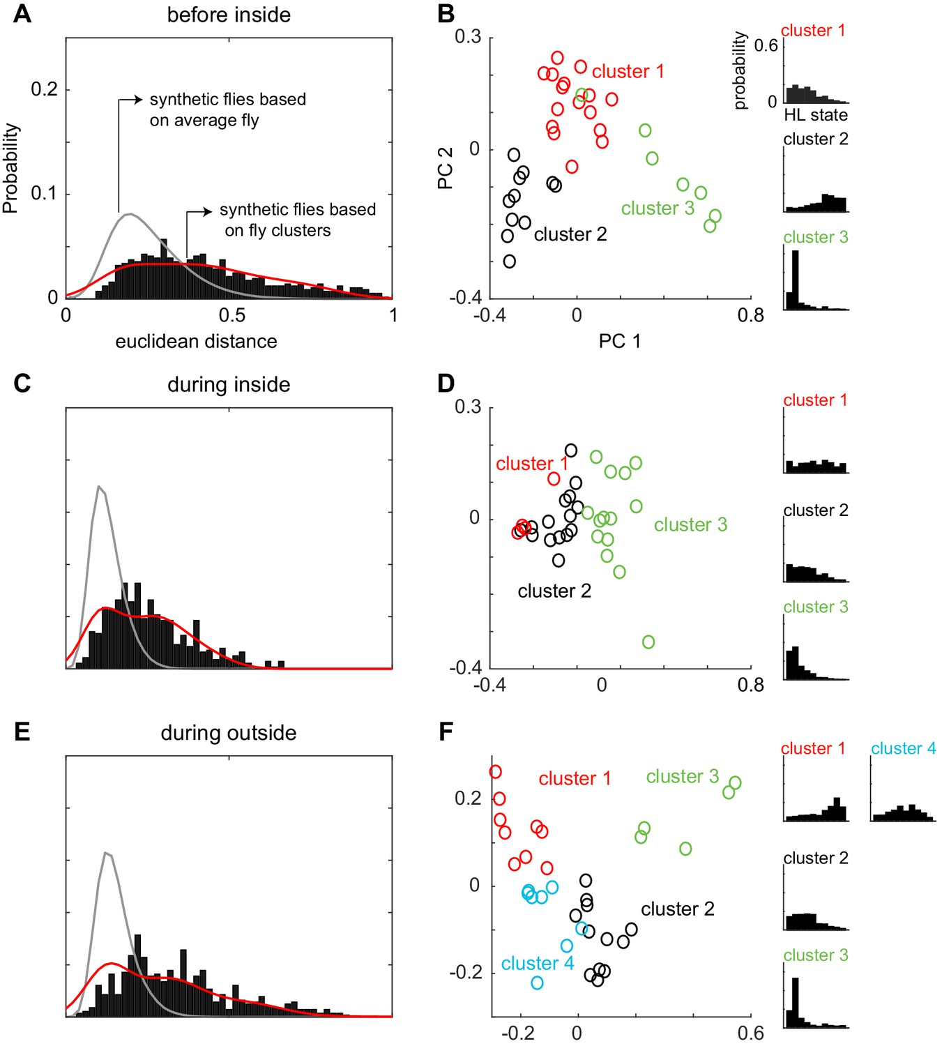
Flies can be clustered into three to four types based on their locomotion.
This figure shows the same analysis as in Figure 7, but for the other three conditions - before inside, during inside and during outside (A) Same as Figure 7A and B, but for "before inside". Average fly (gray line, Wilcoxon rank sum, p < 9.57e-58). Cluster fly (Wilcoxon rank sum, p < 4.13e-3). (B) X-means clustering (a variant of K-means) based on the 10-dimensional space formed by the HL states show that there are three clusters of flies in the ‘before inside’ section. The first two PCs are shown for visualization. Each cluster is represented by a different color. Average HL state distribution for each cluster is shown on the right. (C and D) Same as A and B but for ‘during inside’. Average fly (Wilcoxon rank sum, p < 3.25e-86). Cluster fly (Wilcoxon rank sum, p < 0.019). (E and F) Same as A and B but for ‘during outside’. Average fly (Wilcoxon rank sum, p < 2.42e-130). Cluster fly (Wilcoxon rank sum, p < 2.40e-10).
Figure 7—figure supplement 4
Cluster assignments are stable over time.
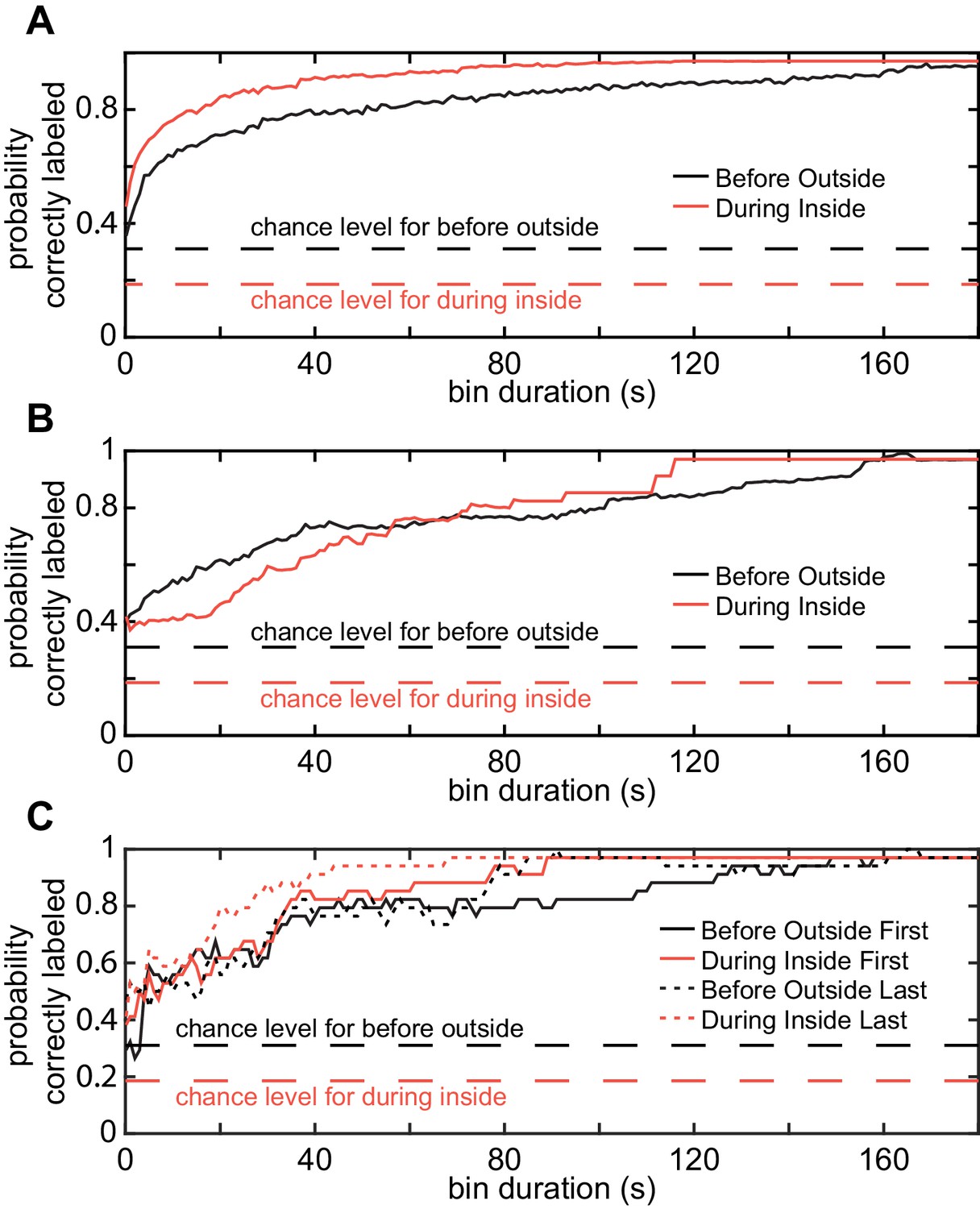
The Euclidean distance between the HL state distribution for each time bin and each of the four centroids were calculated. ‘Correct label’ means that the orginial cluster was the closest. The three panels differed in how the bins were assembled. (A) Probability of assignment to the original cluster based on randomly selected sample. This analysis measures the extent to which subsampling is likely to result in flies in the same cluster. (B) Contigous tracks of given size anywhere in the track show similar assignment stability. (C) Same as C but for the bins at the start and end. Dashed lines represent random chance for before outside (black) and during inside (red).
Figure 7—figure supplement 5
Locomotion before odor onset is only weakly predictive of locomotion during the presence of odor.
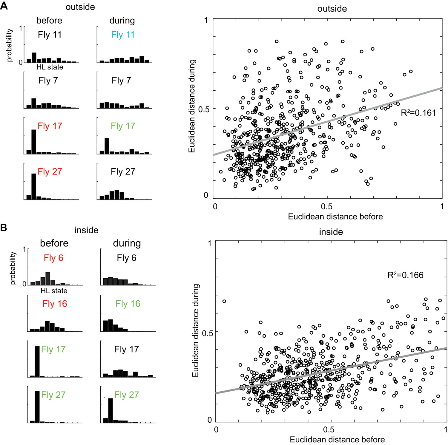
(A) Left: X-means clustering algorithm based on the average HL state distribution for each fly before the odor period and inside the odor ring grouped the 34 flies into three different clusters. Flies belonging to the same cluster, like 11,7 and 17,27 showed similar HL state distributions. The same algorithm grouped the flies in three different clusters during the odor period and inside the odor ring. The flies which belong to the same cluster before the odor period belong to different clusters following odor and show very different HL state distributions from each other. Right: Linear regression analysis between the Euclidean distances before and during the odor period outside the odor ring shows that they are weakly correlated with a r-squared value of 0.161 (p < 0.001). (B) Left: The same analysis was applied to the inside odor case. Again, flies belonging to the same cluster 6,16 and 17,27 before first entry showed different distribution of HLS usage following odor. Right: Linear regression analysis between the Euclidean distances before and during the odor period inside the odor ring shows that they are weakly correlated with a r-squared value of 0.166 (p < 0.001).
Figure 8 with 1 supplement
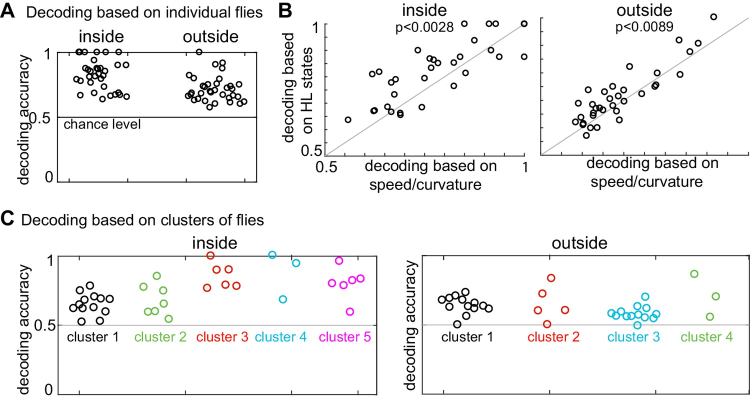
Presence of odor can be decoded based on both HL state distribution of individual flies and clusters of flies.
(A) HL states are a good predictor of whether a fly is experiencing odors. Results of a logarithmic regression (logit) model fit to individual flies consistently shows better probability of correct predictions over chance (grey line). (B) HL states have higher predictive power than speed/curvature for individuals. Logit fits based on HL states were compared to that fit to the speed and curvature for inside (left) and outside (right) of the odor ring. A two-sided Wilcoxon signed rank test showed improved decoding using the HL states (p < 0.0028 for inside and p < 0.0089 for outside).(C) X-means clustering (a variant of K-means) based on the 10 dimensional space formed by the HL states show that there are five clusters of flies for difference in the HL state distributions inside and four clusters of flies for difference in the HL state distributions outside. Results of the logistic regression model fit to these clusters for the inside and outside cases are shown. Each cluster is represented by a different color.
Figure 8—figure supplement 1
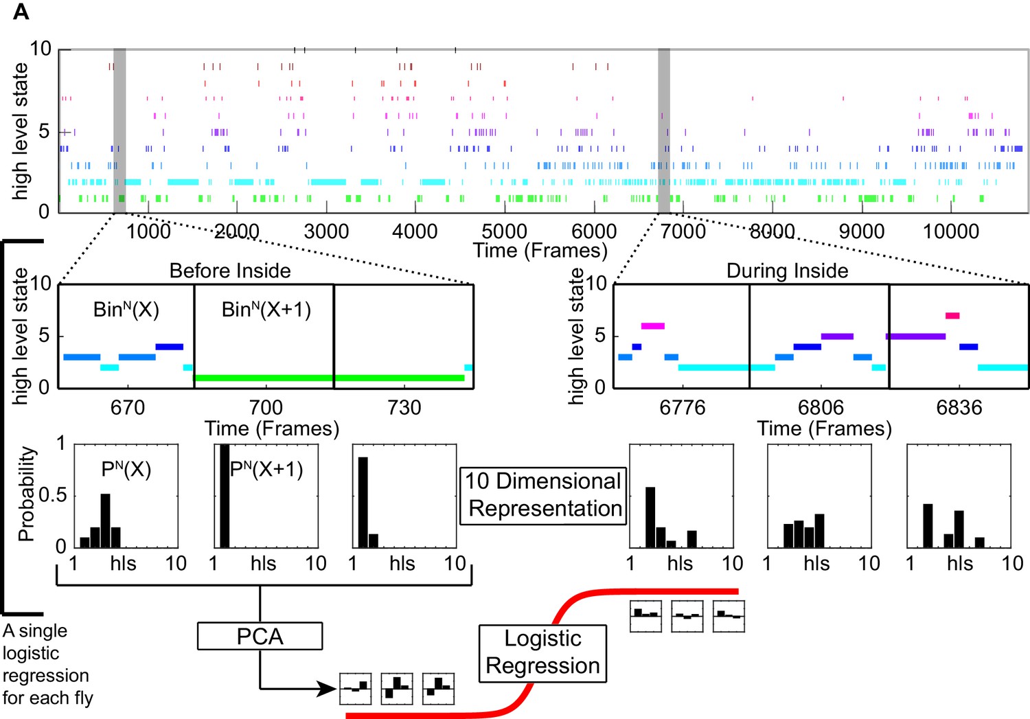
Schematic showing how logistic regression for a single fly was performed.
(A) An example of a high level state track for a fly used in this study. The high level states were separated based on inside and outside the odor ring. For each scenario, the time series was further subdivided into before odor and following first entry. These tracks were divided into segments of 30 frames (1 s) each. The high-level state distributions were calculated for each segment. PCA was applied and the principal components that explains most of the variance were used to fit to a logistic regression (logit) model.
Figure 9
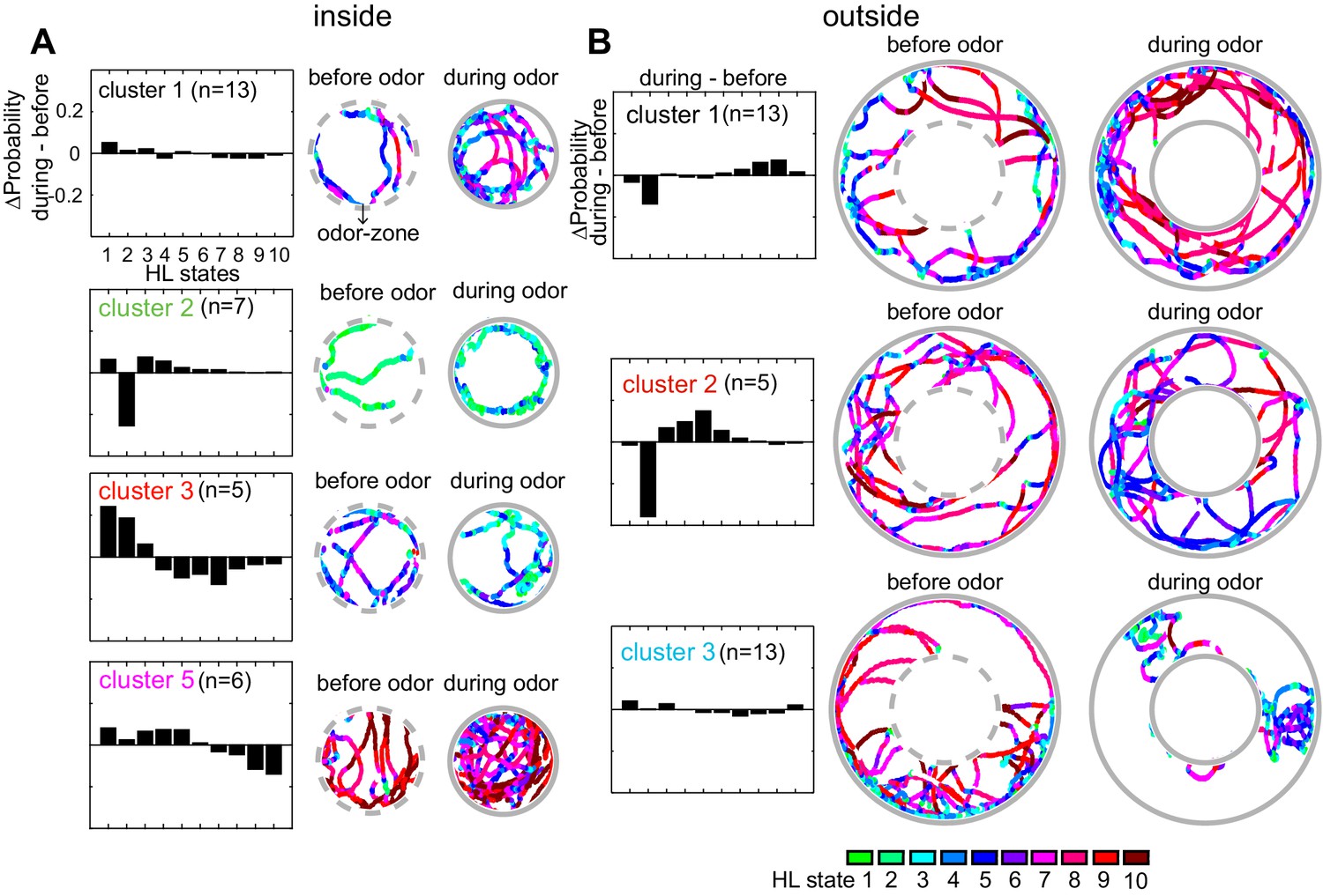
Flies’ response to odors cluster into a small number of distinct, sometimes opposing response-types.
(A) The difference between HL state distributions (during-before) and tracks from an exemplar fly from each cluster is shown. Dotted grey circle indicates the odor-zone. (B) Same as A, but for odor-evoked changes outside the odor-zone.
Author response image 1
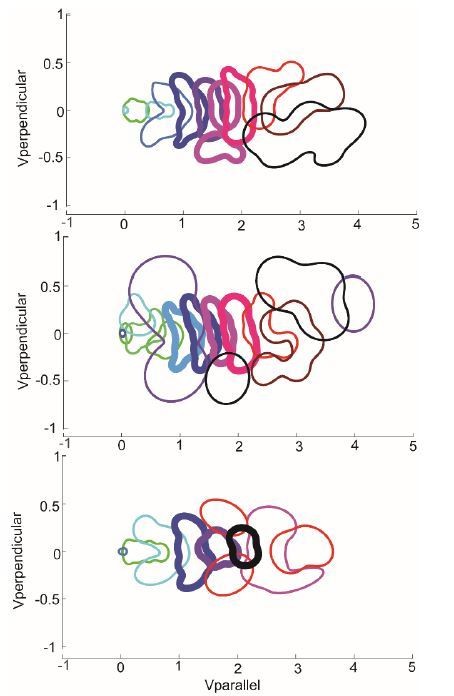
The probability distribution of HL states from 3 models with different number of states – 10 state (top), model described in the manuscript), 12 states (middle), and 8 states (bottom).
The number of middle speed states is the same between the 10-state model and the 12-state model, and decreases by 1 in the 8-state model.
Additional files
-
Transparent reporting form
- https://doi.org/10.7554/eLife.41235.027
Download links
A two-part list of links to download the article, or parts of the article, in various formats.
Downloads (link to download the article as PDF)
Open citations (links to open the citations from this article in various online reference manager services)
Cite this article (links to download the citations from this article in formats compatible with various reference manager tools)
Statistical structure of locomotion and its modulation by odors
eLife 8:e41235.
https://doi.org/10.7554/eLife.41235


