Brain signatures of a multiscale process of sequence learning in humans
Figures
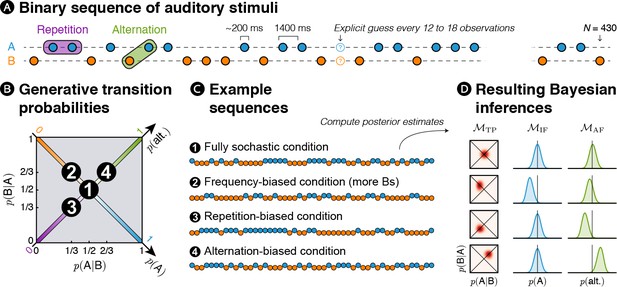
Experimental design: transition probabilities induce orthogonal variations of item frequency and alternation frequency.
(A) Human subjects were presented with binary sequences of auditory stimuli. Each sequence was composed of a unique set of syllables (e.g. A = /ka/ and B = /pi/) presented at a relatively slow rhythm (every 1.4 s) and occasionally interrupted by questions asking subjects to predict the next stimulus. (B) Stimuli were drawn from fixed generative transition probabilities p(A|B) and p(B|A) that varied across four blocks. Those transition probabilities, in turn, determined item frequency p(A) and alternation frequency p(alt.). (C) Example sequences derived from generative transition probabilities used in each condition. The resulting sequences were either fully stochastic, biased toward one of the stimuli (here Bs), or biased toward repetitions or alternations. (D) Learning models were applied to these sequences: a model learning transition probabilities (TP), one learning the frequency of items (IF) and one learning the frequency of alternations (AF). Note that only the TP model can discriminate all four conditions; the IF model is blind to biases toward repetitions or alternations, while the AF model is blind to biases in the balance between stimuli.
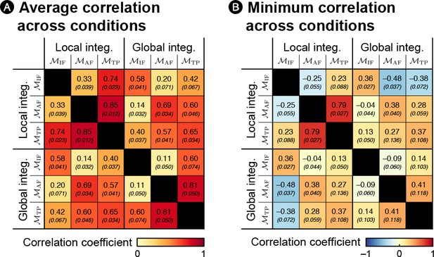
Diagnostic value of the experimental design.
The design aims at identifying both the statistics that are inferred by the brain and the associated timescale of integration. The different conditions have been chosen so as to ensure differences between the theoretical surprise levels of the different learning models (i.e. learning different statistics over different timescales). For instance, in both the frequency-biased and repetition-biased conditions, one item is locally more frequent than the other, but it is true globally only in the frequency-bias condition. Learners inferring the IF based on very local or more global scales of integration will therefore markedly differ between those two conditions. Other differences between models exist in the other conditions. To quantify the diagnostic value of the design, we computed the correlation between theoretical surprise levels estimated from sequences generated randomly according to the four transition probabilities of our design (using 1000 sequences per condition). In the subplot (A), the correlation coefficients are computed after pooling together all conditions. In the subplot (B), the correlation coefficients are computed separately for each condition, and we report the smallest value. The values in brackets indicate the standard deviation across simulations. Altogether, the simulation shows that our experimental design was able to dissociate, in at least one diagnostic condition, the statistics (IF, AF or TP) and their timescale of integration (‘global’ refers to a perfect integration, ‘local’ corresponds to a decay factor ω = 6).
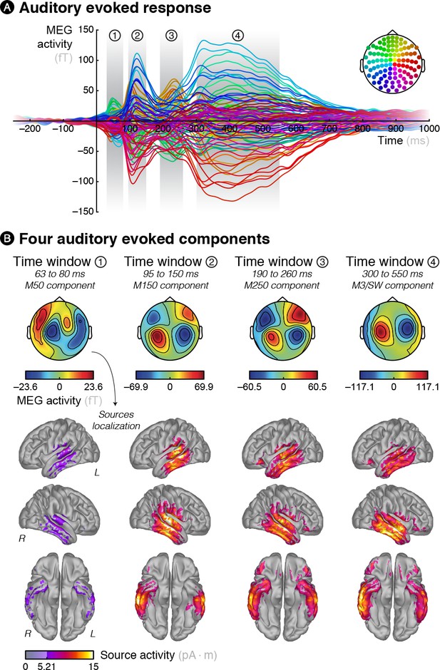
Brain responses evoked by the auditory stimuli.
(A) Grand averaged MEG activity evoked by the auditory stimuli reveals four distinct components. (B) Topographies and source reconstruction of the four components reveal well-known auditory-induced brain activity encompassing early evoked components such as the M50, M150 and M250 and late ones such as the M3 and slow-wave.
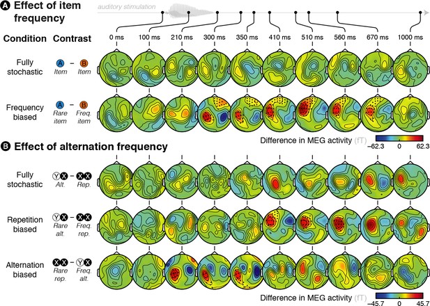
Brain responses are modulated by global statistics.
(A) Difference in brain activity evoked by the two different items in the fully stochastic (in which both stimuli are equiprobable) and frequency-biased (in which one of the two stimuli is more frequent than the other) conditions. (B) Difference in brain activity evoked by alternations and repetitions in the fully stochastic (in which repetitions and alternations are equiprobable), repetition-biased (in which repetitions are more frequent than alternations) and alternation-biased (in which alternations are more frequent than repetitions) conditions. X/Y denotes a pooling of both stimuli together, XX (or YY) thus denotes repetitions of A or B (i.e. AA and BB pooled) while XY (or YX) denotes alternations between A and B (i.e. AB and BA pooled). We report the difference in the MEG responses elicited by a given item (X = A or B) when it is preceded by the same (XX = AA or BB) versus a different (YX = BA or AB) item. Sensors marked with a black dot showed a significant difference (p < 0.05 at the test level and p < 0.05 at the cluster level).
-
Figure 2—source data 1
Violation of global statistics.
Clusters were defined at the group-level with a significance level p < 0.05 (two-sided t-test) uncorrected, at each sensor and time point. We estimated with permutations the significance of those clusters, thereby effectively correcting for multiple comparisons over sensors and times points (Maris & Oostenveld, 2007). The table lists all clusters significant at the level p < 0.05.
- https://doi.org/10.7554/eLife.41541.008

Time courses of the differences between frequent and rare events in the biased conditions.
MEG activity averaged over significant sensors (reported in Figure 2) is plotted as a function of time for both kinds of events (frequent one and rare one) in the three biased conditions, thereby unravelling the dynamics of surprise for (A) rare items, (B) rare alternations and rare repetitions.
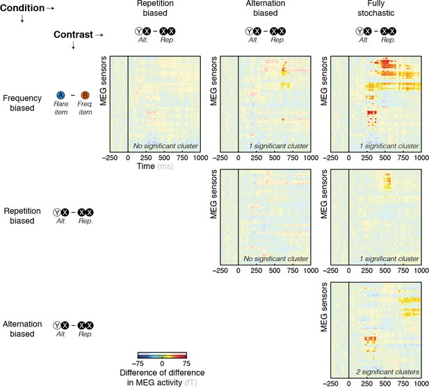
Contrasts between surprise responses across conditions.
Surprise response to global statistics (globally rare – frequent events) at the level of topographies were different between pairs of conditions. Highlighted parts of the sensors x time matrices reflect significant spatio-temporal clusters (p < 0.05 at the test level and p < 0.05 at the cluster level).
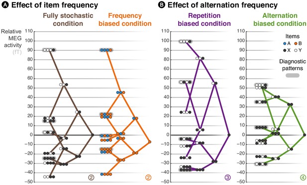
Brain responses are modulated by local statistics.
The brain response to a given observation is plotted as a function of the recent history of events. We connected the possible extensions from shorter to longer patterns, such that the data are represented as a ‘tree’. Each of these trees corresponds to an experimental condition. At each node of a tree, the circles should be read from left to right and denote the corresponding patterns; for instance, the pattern AAAB shows the activity level elicited by the item B when it was preceded by three As. X and Y denote the pooling of both stimuli in conditions in which both stimuli are equiprobable. In the frequency-biased condition, we report the activity evoked by item B, the most frequent stimulus. Activity levels across sensors were averaged using a topographical filter within a late time window (from 500 to 730 ms) post-stimulus onset. The topographical filters were obtained by contrasting rare and frequent patterns (e.g. XYXX – XYXY in the alternation-biased condition). The filters are shown in Figure 3—figure supplement 1; the small, circled and colored numbers at the bottom of each tree serve as identifiers. We defined and applied the filters using a cross-validation approach to ensure statistical independence (see Materials and methods).
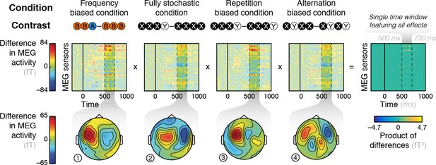
Responses to the violation of local patterns used as spatial filters.
Contrasts between diagnostic patterns that were either violated or continued, for each condition. The topographies are averaged in a late time window (from 500 and 730 ms) that exhibits all effects.
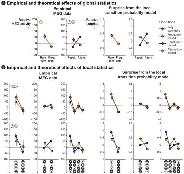
The local transition probability model accounts for modulations of late MEG signals.
Observed MEG signals and theoretical surprise levels predicted by the transition probability model (with a local integration, ω = 6) in response to (A) globally rare events and to (B) violation or continuation of local patterns. MEG signals correspond to activity levels across sensors were averaged using a topographical filter (see Figure 3—figure supplement 1) within a late time window (from 500 to 730 ms) post-stimulus onset. The patterns reported here correspond to the diagnostic ones that are highlighted in Figure 3. See Figure 4—figure supplement 1 for theoretical predictions by other models.
Qualitative account of experimental effects by rival models.
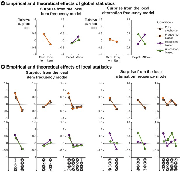
Theoretical surprise levels from the item frequency and alternation frequency models (with a local integration, ω = 6) in response to (A) globally rare events and to (B) violation or continuation of local patterns. The local patterns reported here correspond to diagnostic ones that are highlighted in Figure 3. Surprise levels from the transition probability model is presented along empirical data in Figure 4. Both IF and AF models fail to account for some key aspects of the data. For instance, the IF model does not reproduce the modulation of MEG signals by globally rare repetitions/alternations and the violation of local pattern of alternations. Conversely, the AF model does not reproduce the modulatory effect of frequent/rare items and the violation of local pattern of repetitions.
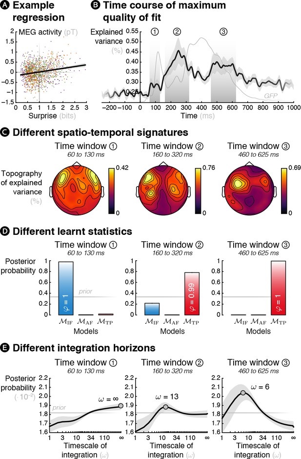
Theoretical surprise levels from learning models fitted to MEG signals reveal a multiscale inference process.
Mass-univariate (across sensors and time points) trial-by-trial regressions of MEG signals against theoretical surprise levels from learning models learning different statistics with different timescale of integration (ω). (A) Example trial-by-trial regression (the colors represent the different conditions), for one subject, at one particular time point, in one particular sensor in the case of transition probability learning with ω = 16. (B) The maximum R2 over models and parameters was averaged across sensors, and then across subjects. The resulting time course reveals three distinct time windows in which regressions yield a high proportion of explained variance. For reference, the thin grey line represents the global field power evoked by all the sounds (see Figure 1—figure supplement 2A). (C) Average topography of maximum R2 values in each time window. (D) Bayesian model comparison reveals that different models best explain MEG signals in these three time windows: item frequency (IF) in an early time window, and transition probabilities (TP) in later time windows. (E) Bayesian model averaging further reveals that different timescales of integration are involved: slow, global integration for the early time window, and increasingly local integration for the later time windows. These posterior distributions give the probability of ω given the MEG data. The error shading shows the inter-subject s.e.m.
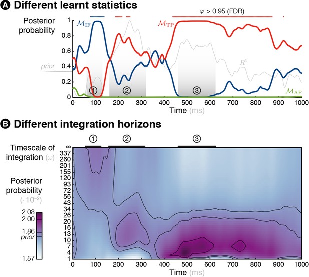
Time-resolved model comparison.
Model comparison and parameter estimation similar to Figure 5 but here in continuous time (and not handpicked time windows, highlighted with circled numbers) after applying a moving average of 80 ms on the MEG evoked response. (A) Bayesian model comparison reveals that different models best explain MEG signals: the learning of item frequency for early responses and of transition probabilities for medium and late responses. (B) Bayesian model averaging reveals that different timescales of integration are involved: from global integration for early responses to more and more local integration for medium and late responses.
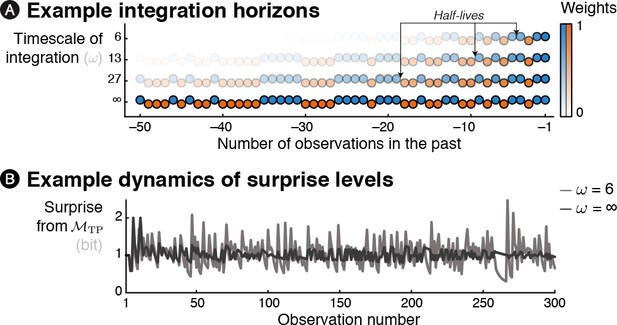
Characteristics of the free parameter controlling the timescale of integration.
(A) Influence of the parameter ω controlling the timescale of integration on the weights attributed to previous observations on the current inference process. For the sake of illustration, the weights are depicted here are transparency levels for a short example sequence. (B) Different timescales of integration translate into different dynamics of surprise levels. Note that when ω parameter is small, the inference is more local and thus results in higher fluctuations of surprise levels throughout the sequence (even after hundreds of observations) in this fully stochastic sequence.
Movie of R2 topographies.
https://doi.org/10.7554/eLife.41541.016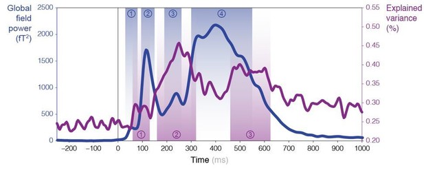
Additional files
-
Transparent reporting form
- https://doi.org/10.7554/eLife.41541.017


