Can Hamilton’s rule be violated?
Figures
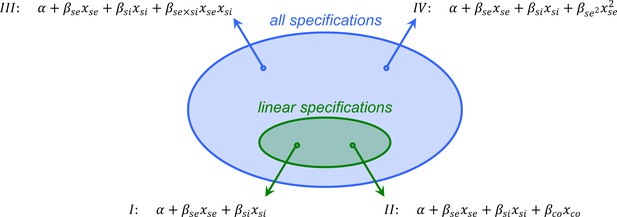
The value of coefficients and may depend on the specification chosen.
If is included (as in specification II), these values will be different from when is not included (specification I). Including an interaction term (III) or a quadratic term (IV) will also make a difference for the value of and . All specifications that are linear, result in Hamilton’s rules, all of which agree with the direction of selection. Hamilton’s rule with specification I says that if and only if – where is the value of , and is minus the value of in this specification. Hamilton’s rule with specification II says that if and only if – where is the value of , is the value of , and is minus the value of in this specification.
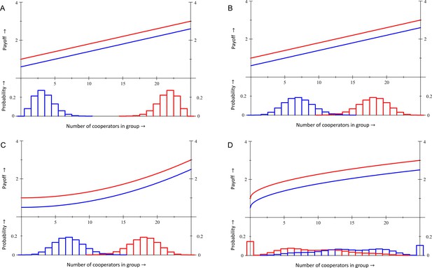
Within each panel, the fitness functions are depicted in the upper part.
In panels A, B and C the bottom part depicts population structure profiles of mutant co-operators at (blue) and of mutant defectors at (red). In panel D the bottom part depicts the distribution of what group types co-operators (blue) and defectors (red) find themselves in, both at the same intermediate equilibrium value for . No violations of Hamilton’s rule with equal gains from switching. In panels A and B, the fitness function is and . In panel A the difference in average fitness between co-operators and defectors is , both at and at . Cooperation therefore is selected against at both ends. Inclusive fitness is also at both ends. Panel B has a more assorted population structure, for which this difference, as well as inclusive fitness, is at both ends, and cooperation is selected for. No violations in equilibrium with synergies. Panel C has the same population structure profiles as panel B, but a different fitness function: and . Here cooperation is selected against at , where , and selected for at , where . Inclusive fitness is at and at . Violation in a mixed equilibrium. In panel D, the fitness function is and . Here, at – which makes it an equilibrium – while inclusive fitness is . Details are in Appendix 1, as are computations of inclusive fitness with costs and benefits according to the regression method instead of the counterfactual method.
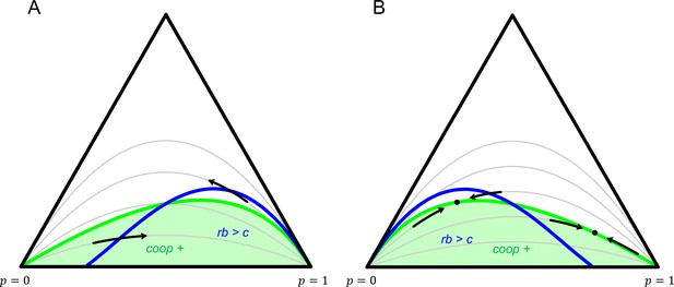
Dynamics for two 2-player games.
Every point in the simplex represents a population state . The left down corner is , which has only groups with co-operators; the right down corner is , which has only groups with co-operators; the top corner is , which has only groups with co-operator. The grey lines represent different population structures, all with constant relatedness. Any given grey line gives a population state for every overall frequency of co-operators. Dynamics make populations move along the line that represents the population structure it faces. All grey lines go through the left down corner, where , and the right down corner, where . The straight line on the bottom reflects a totally assorted population that has no mixed groups. The higher up, the more mixed groups there are, and the less assortment there is. The highest up grey line represents a well-mixed population. No violations of Hamilton’s rule in equilibrium with synergies. In panel A, , , and . The regions where cooperation is selected for (green), and where inclusive fitness is positive (blue) are not the same, but selection always takes populations out of the parts where they disagree. Violations with anti-synergies. In panel B , , and . Here populations can settle at mixed equilibria, while inclusive fitness is not . Violations at and are also possible for more extreme choices of .
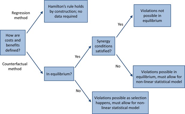
A road map for empirical tests of Hamilton’s rule.
The three synergy conditions are that for all , that for all , and that increases with .
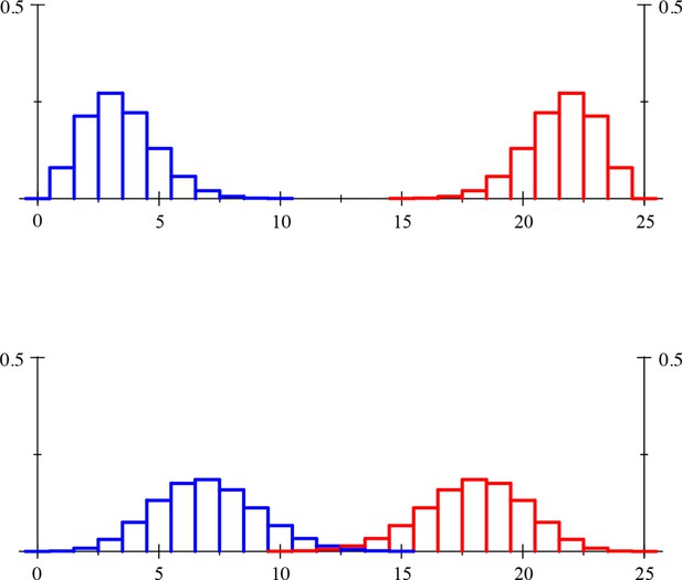
Population structure profiles (blue) for co-operator invaders at , and (red) for defector invaders at .
Defectors at only find themselves in groups with defectors, co-operators at only find themselves in groups with co-operators (not depicted in the figures). In the lower panel mutants assort more than in the upper one, and random matching would result in a population structure profile with single spike at , and a single spike at for . Section IX describes the population structures that result in these population structure profiles. For this population structure is satisfied, which means that the red bars are the mirror image of the blue ones.
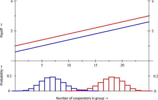
The population structure profiles are depicted in the lower half of the figure, the payoffs in the upper half.
https://doi.org/10.7554/eLife.41901.009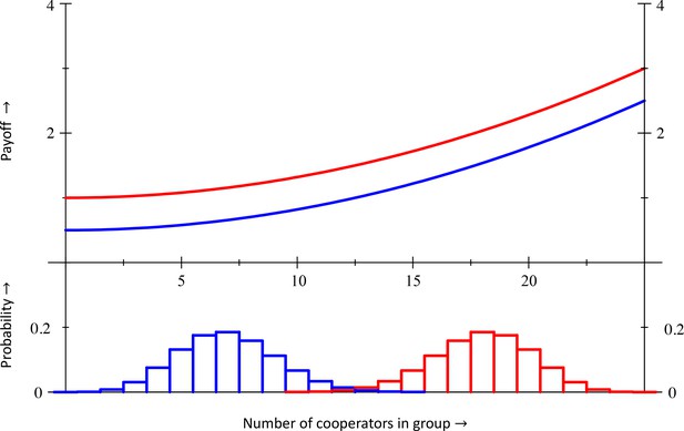
The population structure profiles are depicted in the lower half of the figure, the payoffs in the upper half.
https://doi.org/10.7554/eLife.41901.010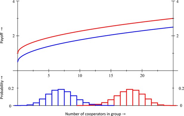
The population structure profiles are depicted in the lower half of the figure, the payoffs in the upper half.
https://doi.org/10.7554/eLife.41901.011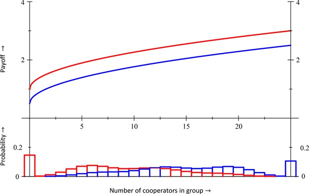
The previous figures depicted , which is the population structure profile at , and , which is the population structure profile at .
The payoffs co-operators get, when they find themselves in groups according to would be compared to the payoffs defectors get when they are in a group of defectors only in order to determine whether co-operators can invade defectors, at , and the mirror image of that in order to determine whether defectors can invade co-operators, at . The and depicted here all pertain to one and the same equilibrium , at which . With the same payoff function as at Appendix 1—figure 4, we find an equilibrium frequency of co-operators of , at which inclusive fitness is .
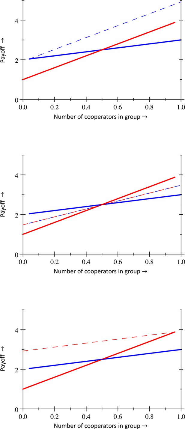
The according to the regression method coincides the true at (top panel, red), but the according to the regression method (dotted blue) differs from the true (solid blue).
The and according to the regression method coincide with each other at (middle panel, dotted lines) but do not coincide with the true (solid red) and (solid blue). The according to the regression method coincides the true at (bottom panel, blue), but the according to the regression method (dotted red) differs from the true (solid red).
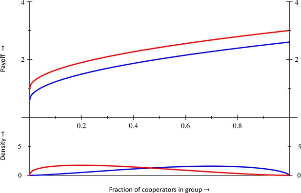
With parameters , and , the equilibrium frequency of co-operators, at which , is .
Inclusive fitness there is . Section X specifies the for this example.
Additional files
-
Transparent reporting form
- https://doi.org/10.7554/eLife.41901.006


