Thalamocortical synapses in the cat visual system in vivo are weak and unreliable
Figures
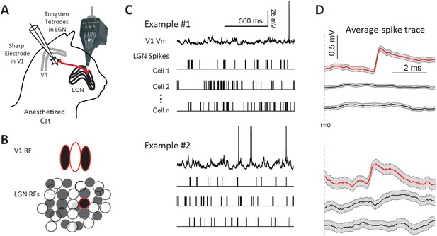
Paired LGN-V1 recordings allow quantification of average thalamocortical EPSPs in connected pairs.
(A) Simultaneous recording of intracellular potentials with a sharp microelectrode from a single V1 neuron and extracellular potentials from many LGN neurons. (B) This allows us to identify one, or more, LGN cells monosynaptically connected to the cortical cell. (C) Sample traces, from two different example experiments, of a V1 cell together with spikes from three simultaneously recorded LGN cells, during the response to white noise. (D) Jitter-corrected spike-triggered average (STA) trace of V1 Vm, and SEM shown in gray, for each LGN cell. The red trace in each panel contains a sharp depolarization indicative of an EPSP from a connected LGN-V1 cell pair. The remaining LGN cells were not connected, exhibiting a flat STA. t = 0 indicates LGN spike time.
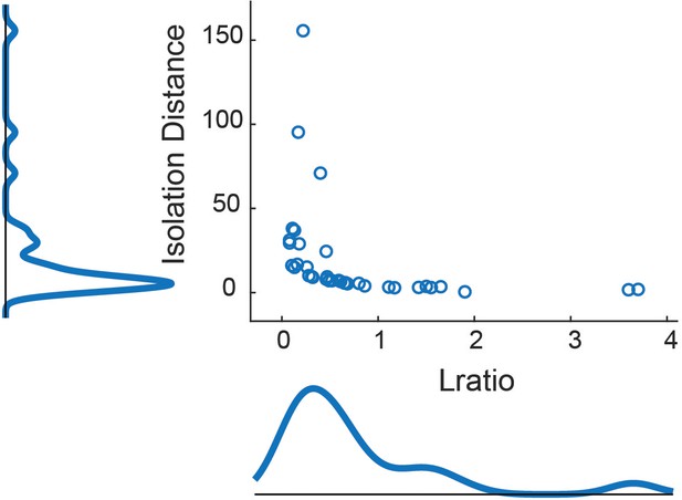
LGN cluster metrics for all connected cells used in this study.
For a description of Lratio and Isolation distance, see Schmitzer-Torbert et al. (2005). The average Isolation distance was 19.3 ± 30.6 (mean ± SD), and the average Lratio was 0.77 ± 0.86. Although many additional features were used to identify clusters, the features used to calculate Lratio and Isolation distance were the energy and first PCA component, as recommended by Schmitzer-Torbert et al. (2005).
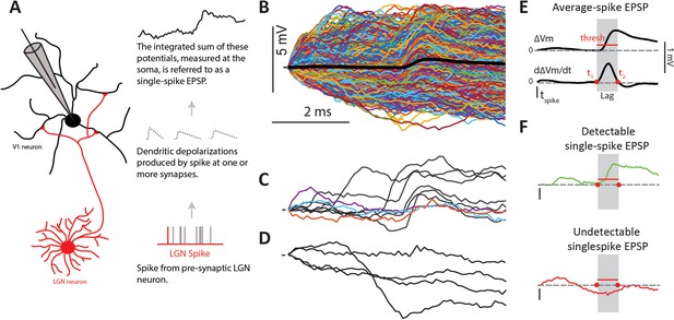
Single-spike EPSPs represent the somatic depolarization produced by a pre-synaptic LGN spike.
(A) An LGN axon from a pre-synaptic cell makes synaptic contacts with its target L4 cell, and therefore causes dendritic depolarizations, which are integrated at the soma. We measure this integrated depolarization with a sharp intracellular electrode. (B) Single-spike traces (n = 2074) for a sample connected pair, overlaid with their average in black. (C) Subset of single-spike traces from B) exhibiting a clear EPSP (black traces), and those without a clear EPSP (colored traces). (D) Subset of single-spike traces from B) that lack a detectable EPSP. (E) The average EPSP and its first derivative are used to determine parameters for the single-spike EPSP detector (see text). The gray region indicates the ‘monosynaptic window’, or the expected window for a monosynaptic EPSP to occur after an LGN spike. (F). Example traces categorized as detectable single-spike EPSP (top) and undetectable single-spike EPSP (bottom).
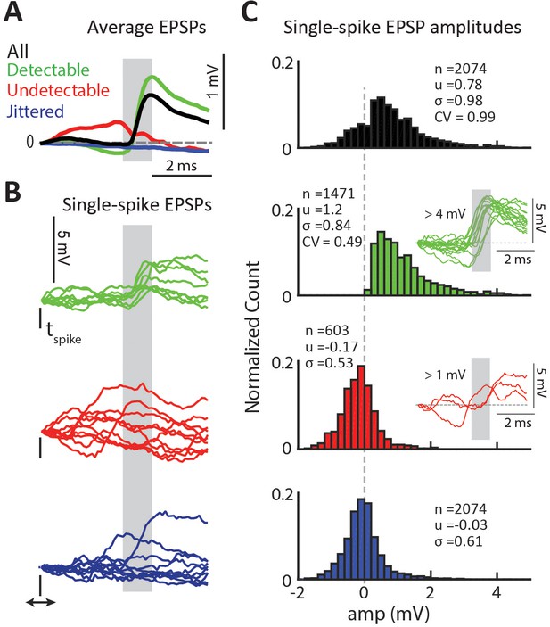
Properties of detectable and undetectable single-spike EPSPs for an example connected pair.
(A) Average EPSP for different spike-categories within the same connected pair. Colors used throughout figure. Gray region indicates the monosynaptic window. (B) Example single-spike EPSPs for each category. (C) Distribution of single-spike EPSP amplitudes for each category. The inset in the second row shows sample detectable single-spike EPSPs with amplitudes at the high tail of the distribution,>4 mV. The inset in the third row shows sample undetectable single-spike EPSPs with amplitudes also at the high tail of the distribution,>1 mV.
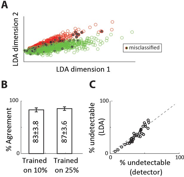
Validating EPSP classification with linear discriminant analysis.
(A) Classification of single-spike EPSPs into detectable and undetectable categories using linear discriminant analysis. The classifier was trained on 10% of single-spike EPSPs that were manually labeled. Misclassifications (black circles) were most often false positives. (B) Percent agreement between categorizations using the automated detector (Figure 2E–F) and linear discriminant classifier, for different fraction of data used as the training set, for the sample connected pair used in Figure 3. (C) Percent of single-spike EPSPs categorized as undetectable for the two methods, for all n = 36 connected pairs.
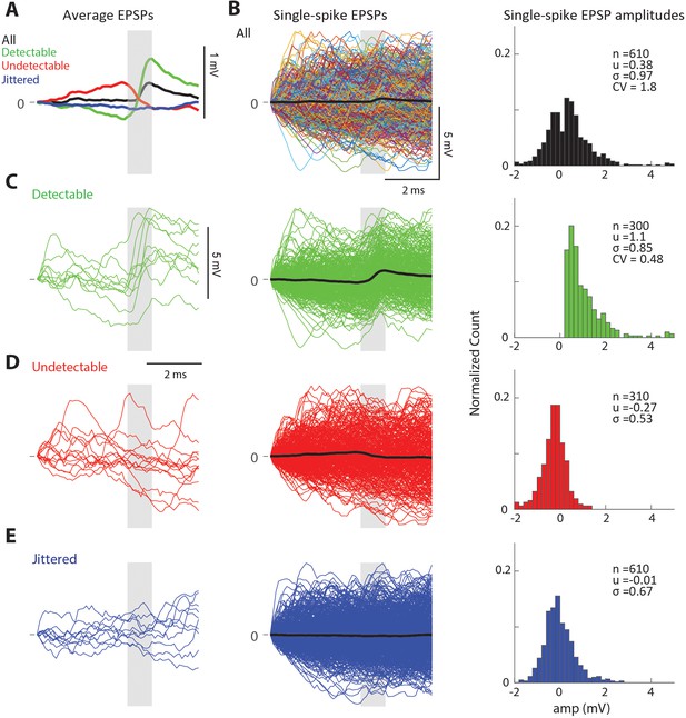
Single-spike traces for an additional sample connected LGN-V1 pair.
(A) LGN spike-triggered average trace of V1 Vm for all spikes (black), successfully transmitted spikes (green) or failed spikes (red)., and jittered spikes (blue). (B) (Left) Average spike-trace (black) overlaid with all n = 610 single-spike traces (top), and separated into spike categories (bottom) as in Figure 1F. (Right) Amplitude distribution of single-spike EPSPs for all four spike categories. (C) Sample single-spike traces categorized as successes, indicated by the presence of a sharp depolarization in the monosynaptic window (gray box). (D) Sample single-spike traces categorized as undetectable single-spike EPSPs. (E) Sample single-spike traces produced by jittered LGN spikes.
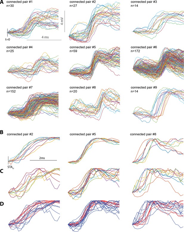
Less common large single-spike EPSPs contain a single sharp depolarization and have a similar shape as the more common small single-spike EPSPs.
(A) Each panel shows the top 1% of single-spike EPSPs with the largest amplitudes. Close inspection of the rising phase of each single-spike EPSP suggests a single smooth and sharp depolarization. t = 0 is the occurrence of the pre-synaptic LGN spike B) A selection of the largest 1% of single-spike EPSPs, normalized to the peak of each trace. To ease visual comparison of the rising phase of the EPSP, traces are shown in a limited 2 ms time-window. STAt1 refers to the onset of the rise of the average STA for each connected pair. Single-spike EPSPs with large negative deviations before the rising phase were removed from these plots to reduce the overall range of the plot and ease visual assessment. Including these traces made visualization difficult but did not change the results. (C) Same as (B) but for single-spike EPSPs in the 20th −25th amplitude percentile. (D) B and C overlaid. Red traces indicate normalized large EPSPs and blue traces normalized small EPSPs.
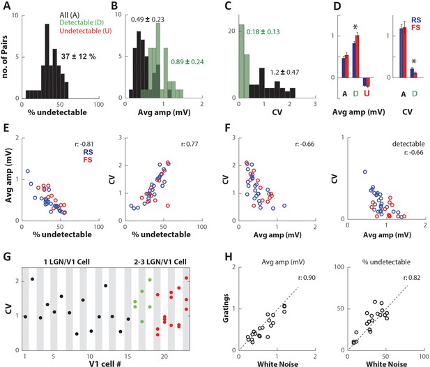
Thalamocortical synapses produce highly variable and unreliable EPSPs.
(A) Distribution of percentage of undetectable single-spike EPSPs (%undetectable) for all n = 36 connected pairs. Numbers indicate mean ± SD. (B) Distribution of average trace amplitude (Avg amp), averaged over all single-spike traces (All (A), black), and only detectable single-spike EPSP traces (Detectable (D), green). (C) Distribution of coefficient of variation (CV) of single-trace amplitudes, calculated from all traces (black), and detectable EPSP traces only (green). (D) (Left) Population average (error bars indicate SEM) of Avg amp for all (A), detectable (D), and undetectable (U) single-spike EPSPs. Blue/red bars within category indicate connections onto regular spiking (RS)/fast spiking (FS) V1 cells. (Right) Population average of CV values for all spikes and detectable EPSPs. (E) (Left) Avg amp decreases with increasing %undetectable. (Right) CV increases with increasing %undetectable. Colors indicate connections onto RS or FS cells. (F) CV decreases with increasing Avg amp for all spikes (left) and for detectable only (right). (G) CV plotted for all n = 36 connected pairs, separated on the x-axis according to the target V1 cell #. Black/green/red indicates V1 cells that had 1/2/3 connected LGN cells in our dataset. (H) Avg amp and %undetectable for a subset of connected pairs during response to white noise vs. drifting gratings.
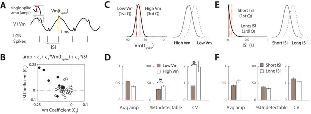
Factors that influence synaptic variability.
(A) For each LGN spike, the amplitude of the single-spike trace (amp) was correlated with the instantaneous Vm driving force (average Vm in 1 ms window around spike time, see Materials and methods) and the inter-spike-interval (ISI). (B) This data was fit to a linear regression model separately for each n = 36 cell pairs. A fraction of cells (9/36) cell pairs exhibited significant regression coefficients for Vm and ISI (black circles). (C) Schematic showing categorization of instantaneous driving force associated with each spike into low (hyperpolarized) and high (depolarized) Vm based on quartiles of the probability distribution. (D) Population average across all connected pairs of different synaptic parameters during low Vm and high Vm categories. Error bars indicate SEM. * indicates significant (p<0.05) difference in group averages. (E) Same as C, but for ISI. (F) Same as D, but for ISI categories.
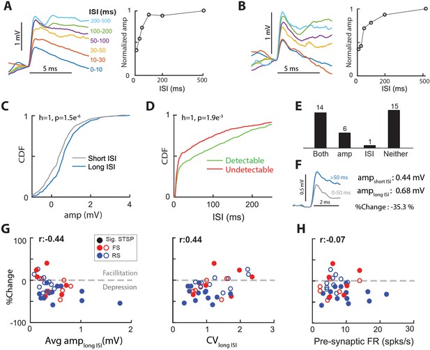
Thalamocortical synapses exhibit short-term synaptic plasticity.
(A) (Left) Average EPSPs grouped by inter-spike-interval (ISI) for a sample connected pair. (Right) Normalized EPSP amplitude vs. ISI for the same connected pair. (B) Same as A, for another sample connected pair. (C) Cumulative distribution functions (CDF), of single-spike EPSP amplitude distribution for spikes with short (0–50 ms) ISI and those with long (>50 ms) ISI, for the connected pair in A. p values are from 2-sample KS test. (D) CDFs of ISI distribution for detectable and undetectable single-spike EPSPs, for the sample connected pair in A. (E) No. of synapses with separable distributions for both, just EPSP amp for short and long ISIs, just ISI for detectable and undetectable EPSPs, or neither. Most synapses with a separable distribution of EPSP amplitudes for short and long ISIs, also exhibited separable ISI distributions for detectable and undetectable EPSPs. (F) STSP was quantified as the % change in average EPSP amplitude for long-ISI EPSPs, relative to short-ISI EPSPs. (G) (Left) % change of average EPSP amplitude with ISI as a function of the long-ISI average EPSP amplitude for all connected pairs. Filled circles indicate significant STSP. (Right) %change plotted against CV of the amplitude distribution for long-ISI EPSPs. (H) %change plotted against the firing rate of pre-synaptic LGN cell.

Pre-synaptic firing rate is not correlated with synaptic variability or reliability.
(A) Average trace EPSP amplitude (Avg amp) as a function of the connected pre-synaptic LGN cell’s firing rate during the same time-period used to estimate EPSP. (B) Same as A but for %Undetectable. (C) Same as A but for CV.
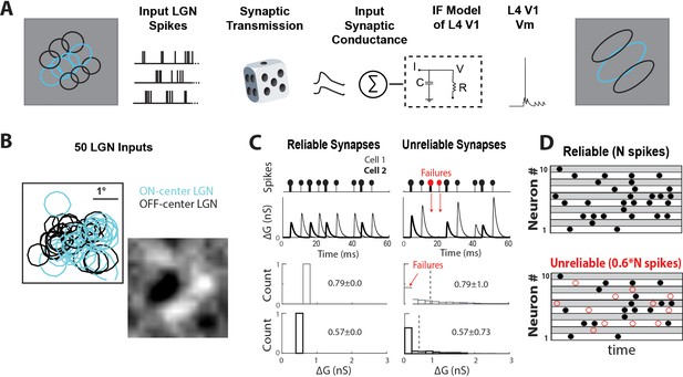
Data-driven feedforward model used to explore effect of thalamocortical synaptic variability and reliability in V1.
(A) Model input:output schematic. Spiking responses, during white noise visual stimulus, of a group of prerecorded LGN cells selected to form a V1-like RF are used as pre-synaptic input for the model. These pre-synaptic inputs undergo either reliable or unreliable synaptic transmission, and are summed to produce a total synaptic conductance to the V1 cell. (B) RF-center contours of the 50 ON and OFF-center LGN cells used as inputs to the model, along with the population RF of all spikes. (C) (Top) Conversion of pre-synaptic spikes into excitatory post-synaptic conductance (EPSG) for model cell with two example reliable (left) and unreliable (right) synapses. (Bottom) Distribution of EPSG amplitudes for a sample synapse under reliable and unreliable model. The distributions have the same mean, but different variance. (D) Schematic showing random selection of ~40% of pre-synaptic spikes designated as undetectable EPSPS (failures, red circles) for each synapse in unreliable model.
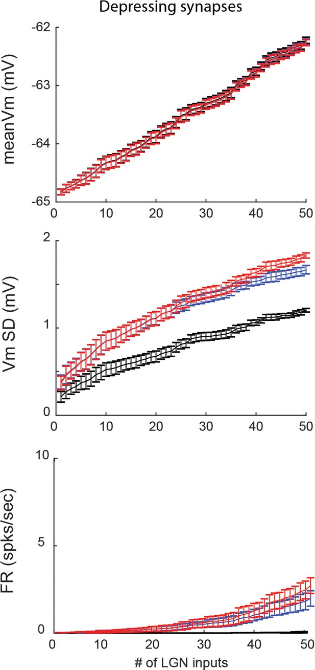
Feedforward model with depressing synapses produces similar results as model without depressing synapses.
(A) Average Vm of model V1 cell as a function of the number of pre-synaptic LGN inputs. Output of the reliable model, and both types of unreliable model with different distribution of failures across the pre-synaptic population are indicated by color. Error bars indicate 95% confidence intervals based on n = 10 trials. (B) Same as A, but for standard deviation of the Vm (Vm SD). (C) Same as A, but for firing rate of the V1 model cell.
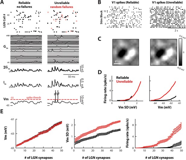
Variable and unreliable synapses boost the thalamocortical drive in a model V1 cell.
(A) Sample 100 ms simulation for the reliable (left) and unreliable (right) model. Undetectable EPSPs are called failures. (Top) LGN Spike inputs for each of 50 synapses, with spike failures shown as red dots. (Middle) Excitatory conductance trace for each synapse, total synaptic conductance, and total current input. (Bottom) Corresponding V1 Vm, which is below spike-threshold for both models. (B) V1 spike rasters for 20 4 s blocks of the white noise stimulus for reliable and unreliable model. (C) Model V1 RFs, at time of pixel with strongest response (75 ms). (D) V1 firing rate as a function of V1 Vm standard deviation (Vm SD, left) and mean (right). Each point represents the average value across n = 10 simulations. (E) Average Vm, Vm SD, and firing rate of V1 cell as a function of the number of synaptic inputs, for n = 10 simulations of the reliable and unreliable model. Error bars indicate 95% confidence intervals.
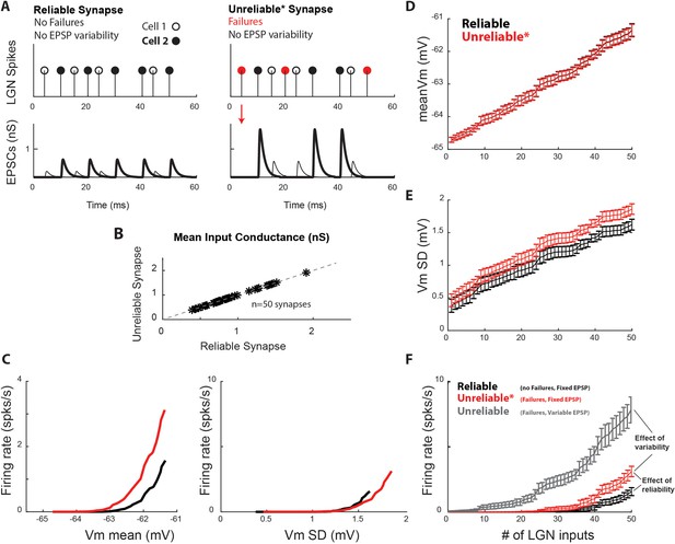
Synaptic variability and unreliability both contribute to increased thalamocortical drive.
To explore the contribution of synaptic reliability alone on cortical spike output, we created a new model with unreliable synapses that exhibited undetectable single-spike EPSPs (‘failures’) but no single-spike EPSP variability (unreliable *). (A) Conversion of pre-synaptic spikes into excitatory post-synaptic conductance (EPSG) for model cell with two reliable (left) and unreliable * (right) synapses. The unreliable synapses exhibit spike failures, but the successful single-spike EPSPs for a synapse all have the same amplitude. (B) To allow for a controlled comparison, the mean conductance input for each of the 50 unreliable synapses (y-axis) was matched with the mean conductance input for the corresponding reliable synapse (x-axis). Dashes show line of equality. (C) V1 firing rate as a function of V1 Vm standard deviation (SD) and mean. Each point represents the average value across n = 10 simulations. (D) Average Vm, (E) Vm SD, and F) firing rate of model V1 cell as a function of the number of synaptic inputs, for n = 10 simulations of the reliable and unreliable* model. For reference, the unreliable model used throughout the paper, which exhibits failures and variable EPSP amplitudes is also shown (gray). Error bars indicate 95% confidence intervals. The firing rate produced by the unreliable* model is higher than that produced by the reliable model, but lower than that produced by the unreliable model with failures and EPSP variability.
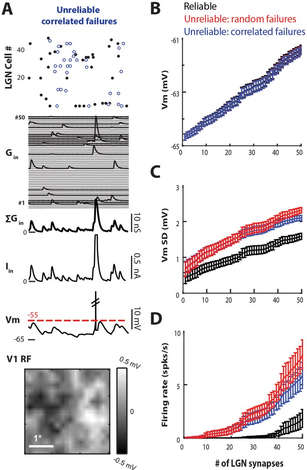
Unreliable synapses with non-random correlated failures also drive cortex better than reliable synapses.
(A) (Top) 100 ms sample of LGN spike-trains for a model with unreliable synapses, with failures (blue dots) that are correlated among LGN cells. Compare to random failures in Figure 7A. (Middle) Excitatory conductance trace for each synapse, total synaptic conductance, total current input, and resulting V1 Vm. (Bottom) RF of V1 cell estimated from the Vm. (B) Average Vm as a function of the number of synaptic inputs, for n = 10 simulations of the reliable (black traces), unreliable with random failures (red traces), and unreliable with correlated failures (blue traces) models. Error bars are 95% confidence intervals. (C) Average VmSD as a function of number of synaptic inputs. (D) Average firing rate of V1 cell as a function of number of synaptic inputs.
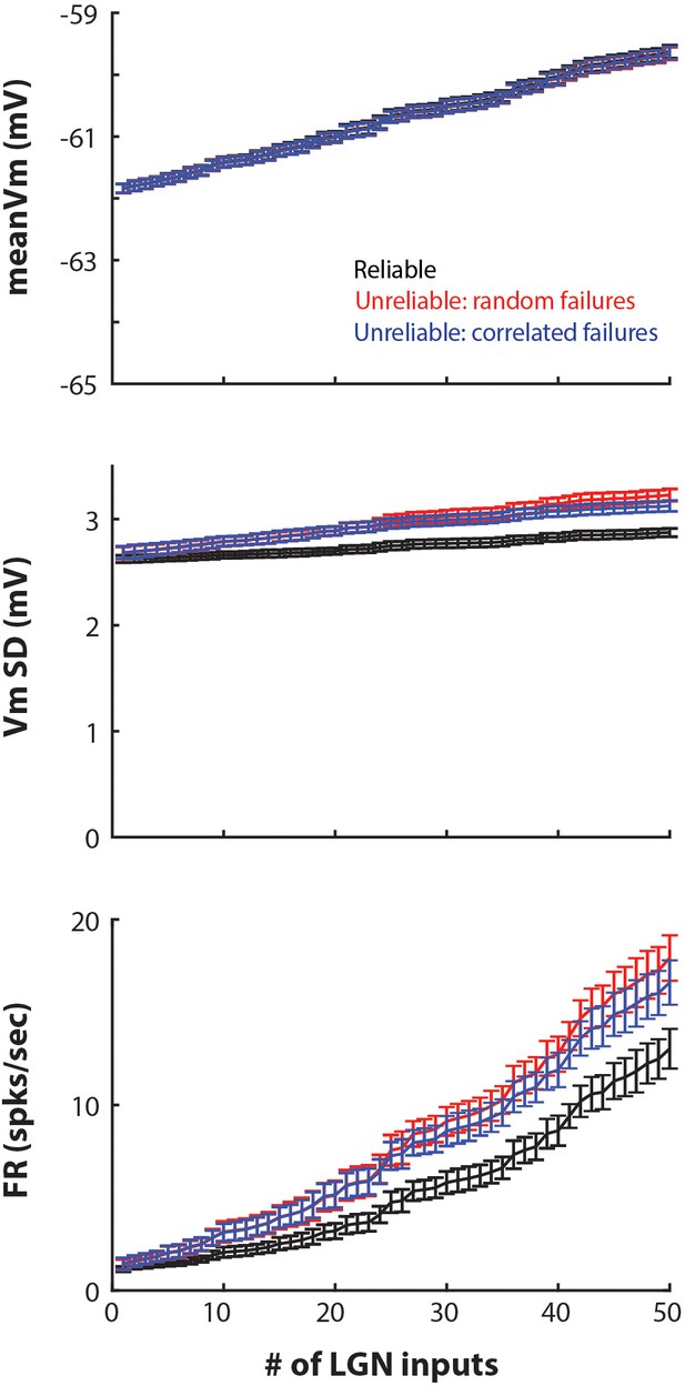
Feedforward model with high conductance state created by adding balanced excitatory and inhibitory background conductance.
Compared to the model with high conductance state created by a low membrane time constant (Figures 6 and 7), this model produced higher cortical firing rates. However, the results were qualitatively the same: unreliable synapses with either random (red traces) or correlated (blue traces) failures produced higher cortical membrane fluctuations and firing compared to reliable synapses. The firing rates observed in vivo are closer to firing rates produced by the model with high conductance state produced by a low membrane time constant (Figure 7).
Additional files
-
Transparent reporting form
- https://doi.org/10.7554/eLife.41925.019


