New tools for automated high-resolution cryo-EM structure determination in RELION-3
Figures
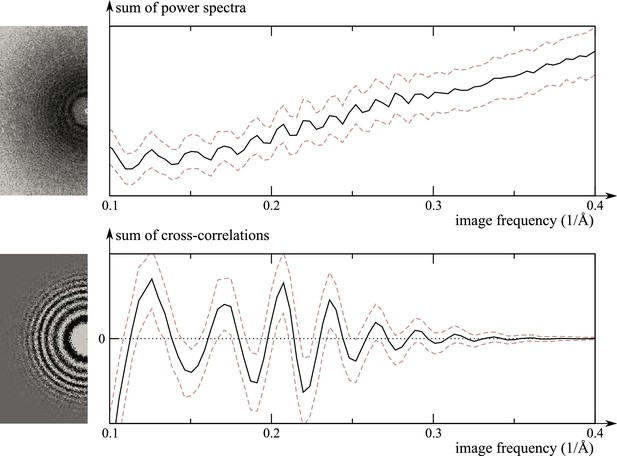
Comparison of the traditional power-spectrum-based CTF estimation technique with reference-map-based CTF refinement.
Top: Sum over the power spectra of all polished particle images in micrograph EMD-2984_0000 of EMPIAR-10061 (left) and the averages and standard deviations of that sum over Fourier rings between 10 Å and 2.5 Å (right). The dashed grey curves are located one std. deviation of each ring above and below the average. The overall rise in spectral power as a function of frequency is a consequence of particle polishing. Bottom: The corresponding plot for the sum over the real components of , instead of the power spectra. Note that the latter term is not only centered around zero, obviating the need to estimate the background intensity, but it also offers a higher signal-to-noise ratio.
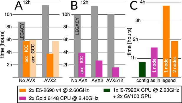
Accelerated CPU performance (A) Even when specific vector instructions are disabled, RELION-3 runs faster than RELION-2 even on the previous-generation Broadwell processors that are ubiquitous in many cryo-EM clusters worldwide.
Enabling vectorisation during compilation with the Intel compiler benefits the new streamlined code path, but not the legacy code. (B) For latest-generation Skylake CPUs, the difference is much larger even with only AVX2 vectorisation enabled, and when enabling the new AVX512 instructions the performance is roughly 4.5x higher than the legacy code path. (C) The accelerated CPU code executing on dual-socket x86 nodes provides cost-efficiency that is at least approaching that of professional-class GPU hardware (but not consumer GPUs).

FCSs comparing half-sets in each type of run, legacy-CPU, acc-CPU, and acc-GPU, all reach the same resolution and sampling accuracy.
Additional FSCs compare the reconstruction of the acc-CPU and acc-GPU using the legacy-CPU as a base of comparison, showing numerical agreement beyond the reconstructed signal threshold. This validates that the quality of results has not been compromised from using lower precision or compiler optimisation.
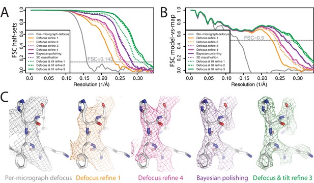
Per-particle defocus correction (A) FSC curves between independently refined half-maps for the different stages of processing as explained in the main text.
(B) As in A, but FSC curves are between the cryo-EM maps and the corresponding atomic model (PDB-4FNK) (Ekiert et al., 2012). (C) Representative density features for some of the maps for which FSC curves are shown in A and B.
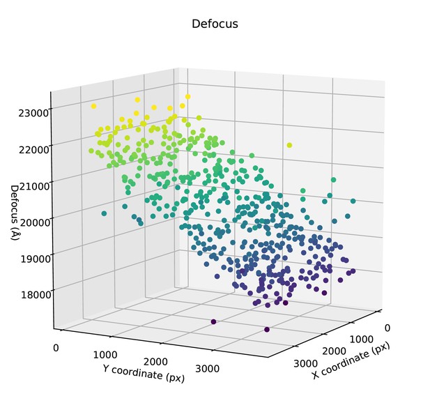
Per-particle defocus estimates (along Z) are plotted against the X,Y-coordinates of the particles in a representative micrograph.
https://doi.org/10.7554/eLife.42166.006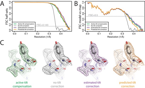
Beam tilt correction (A) FSC curves between independently refined half-maps for the different stages of processing as explained in the main text.
(B) As in A, but FSC curves are between the cryo-EM maps and the corresponding atomic model (PDB-2W0O) (de Val et al., 2012). (C) Representative density features from the 2.2 Å map from the data set with active beam tilt compensation (left); the 2.9 Å map from the data set without active beam tilt compensation and without beam tilt correction (middle); and the 2.2 Å map from the data set without active beam tilt compensation but with beam tilt correction (right).
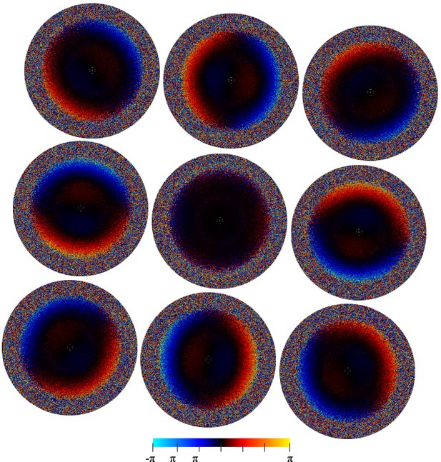
The average per-pixel phase differences (in radiants) between reference projections and the individual experimental particle images (i.e. the phase angle of in Equation 8).
The nine plots correspond to subsets of images collected at the nine different holes without active beam-tilt compensation. Note that the applied beam shift values have been recorded in stage coordinates giving a 175 degree X-axis rotation for the magnification used, which is reflected in the relative position of the nine plots. The inside regions showing the opposite slope to the global trend result from a systematic error in particle alignment caused by beam tilt.

The estimated beam tilt is plotted against the beam-shift values from serialEM in the X-direction (black circles) and in the Y-direction (red circles).
Linear fits through these points indicate there is 0.19 mrad of beam tilt for each m of beam shift.
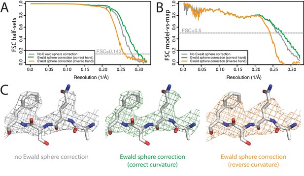
Ewald sphere correction (A) FSC curves between independently refined half-maps without Ewald sphere correction (grey); with Ewald sphere correction with the correct curvature (green) and with Ewald sphere correction with the inverse curvature (orange).
(B) As in A, but FSC curves are between the cryo-EM and the corresponding atomic model (PDB-5UU5) (Hryc et al., 2017). (C) Representative density features without Ewald sphere correction (grey) with Ewald sphere correction and the correct curvature (green) and with Ewald sphere correction and the reverse curvature (orange).
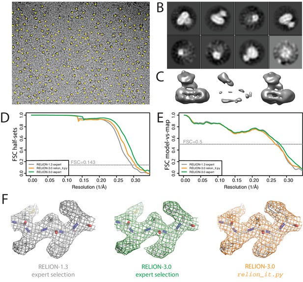
Non-interactive data pre-processing.
(A) Particle positions as selected by the LoG-based auto-picking algorithm are shown as yellow dots. (B) The 2D class averages for the eight largest classes after LoG-based autopicking of the first batch of 10,000 particles. (C) 3D models generated by the script: after SGD initial model generation (left), and after 3D classification for the largest class (middle) and the second largest class (right). The two maps after 3D classification are thresholded at the same intensity level. (D) FSC curves between independently refined half-maps for EMD-3061 (grey), for the map obtained after non-interactive pre-processing (orange) and for the map obtained after processing of the originally published subset of particles in RELION-3. (E) FSC curves between PDB-5A63 and the same maps as in D. (F) Representative density features for the maps in E and F.
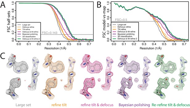
High-resolution refinement: -galactosidase (A) FSC curves between independently refined half-maps for the different stages of processing as explained in the main text.
(B) FSC curves between PDB-5A1A and the maps at the same stages of processing as in A. (C) Representative density features for some of the maps for which FSC curves are shown in A and B.
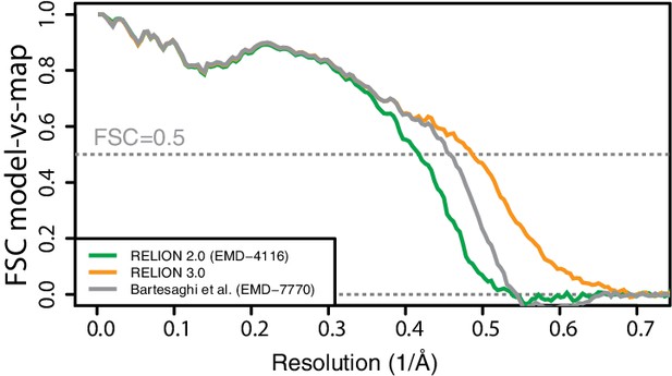
FSC curves between PDB-5A1A and EMD-4116, EMD-7770 and the new map reconstructed in RELION-3.
https://doi.org/10.7554/eLife.42166.013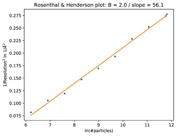
The B-factor plot that was generated automatically by the bfactor_plot.py script.
The script performed nine 3D refinement and post-processing jobs with subsets of increasing sizes for the beta-galactosidase data set. Fitting a straight line through the inverse of the resolution squared of each refinement against the natural logarithm of the number of particles in the corresponding subset yielded an estimated B-factor of 56 Å2.
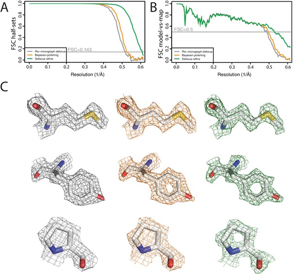
High-resolution refinement: apo-ferritin (A) FSC curves between independently refined half-maps at different stages of the processing.
(B) FSC curves between PDB-5N27 (Ferraro et al., 2017) and the cryo-EM map at different stages of the processing. (C) Representative density features at different stages of the processing.
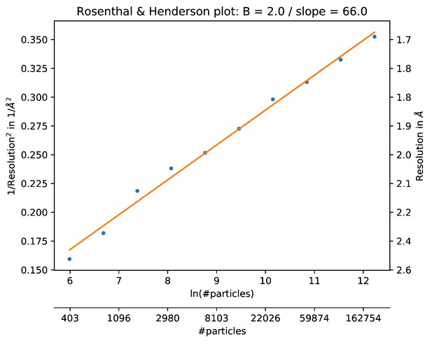
The B-factor plot that was generated automatically by the bfactor_plot.py script.
The script performed ten 3D refinement and post-processing jobs with subsets of increasing sizes for the high-resolution apo-ferritin data set. Fitting a straight line through the inverse of the resolution squared of each refinement against the natural logarithm of the number of particles in the corresponding subset yielded an estimated B-factor of 66 Å2.
Tables
| Reagent type | Designation | Reference | Identifier |
|---|---|---|---|
| software | RELION | Scheres, 2012b | RRID:SCR_016274 |
Additional files
-
Transparent reporting form
- https://doi.org/10.7554/eLife.42166.017


