Figures and data in Spatial control of irreversible protein aggregation | eLife

Figures
Additional files

6 figures and 1 additional file

Figures

Figure 1

Download asset Open asset

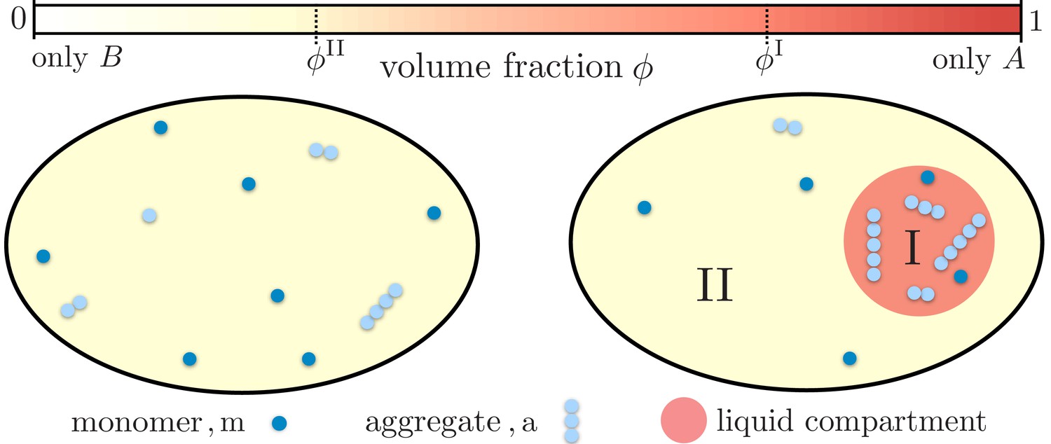
Partitioning of monomers and aggregates via liquid-like compartments.

Protein aggregation may occur homogeneously inside cells also leading to aggregates inside more sensitive cellular regions (left). A liquid compartment may accumulate monomers and thereby trigger the local formation of aggregates (right). The hardly diffusing aggregates are thus kept away from a more sensible cellular region. Such a spatial segregation of aggregates is ideal for adding functional, drug-like molecules which dominantly dissolve inside the compartment. These molecules may degrade the aggregates or inhibit further growth and nucleation. But most importantly, as these molecules are localized inside the compartment their toxic effects are diminished.

https://doi.org/10.7554/eLife.42315.002

Figure 2

Download asset Open asset

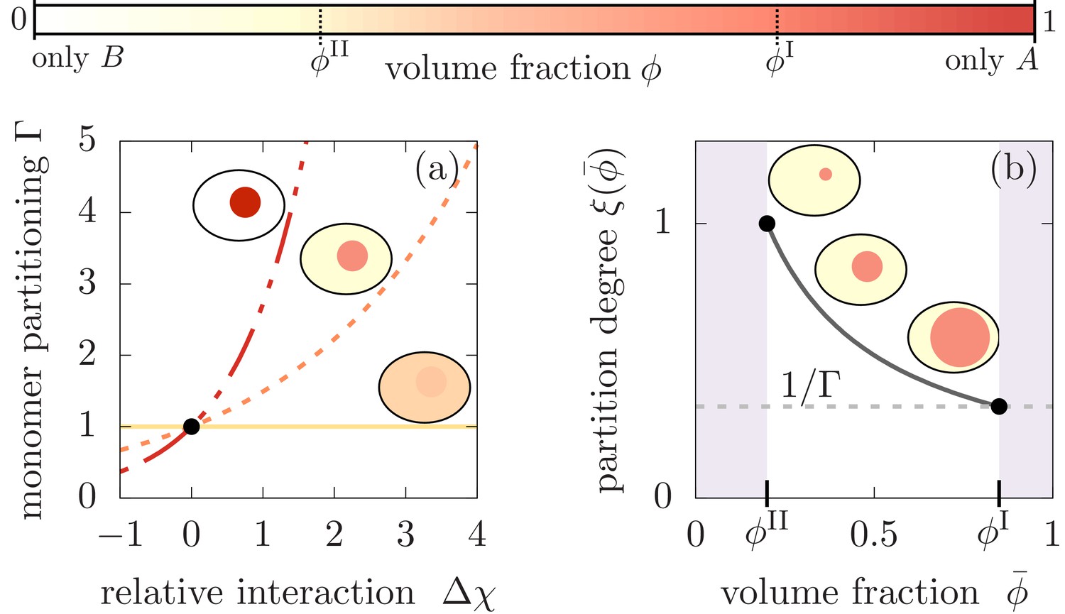
Monomer partitioning and relative degree of segregation.

(a) The monomer partitioning $Γ$ (Equation 1) exponentially increases with the relative interaction strength $Δ χ$ (units of $k_{B} T$ ) between the monomers and the $A$ and $B$ molecules which is defined in the Appendix. Its characteristic increase is set by the degree of phase separation, $ϕ^{I} - ϕ^{I I}$ . Partitioning vanishes at the critical point of phase separation (solid line) and increases with the degree of phase separation (dashed line). Partitioning is largest for $ϕ^{I} - ϕ^{I I} ≃ 1$ (dash-dotted line). Due to the exponential increase, large monomer partitioning $Γ$ can already be reached for weak relative interaction energies of a few $k_{B} T$ . (b) The partition degree $ξ (\bar{ϕ}) = c_{m}^{I I} / c_{m}^{t o t}$ (Equation 2) describing the concentration fraction of monomers that resides in the minority phase II of the compartment, decreases with the mean volume fraction of $A$ material, $\bar{ϕ}$ , along with increasing compartment volume $V^{I} (\bar{ϕ})$ . Smaller compartments are thus better in enriching the monomer mass concentration.

https://doi.org/10.7554/eLife.42315.003

Figure 3

Download asset Open asset

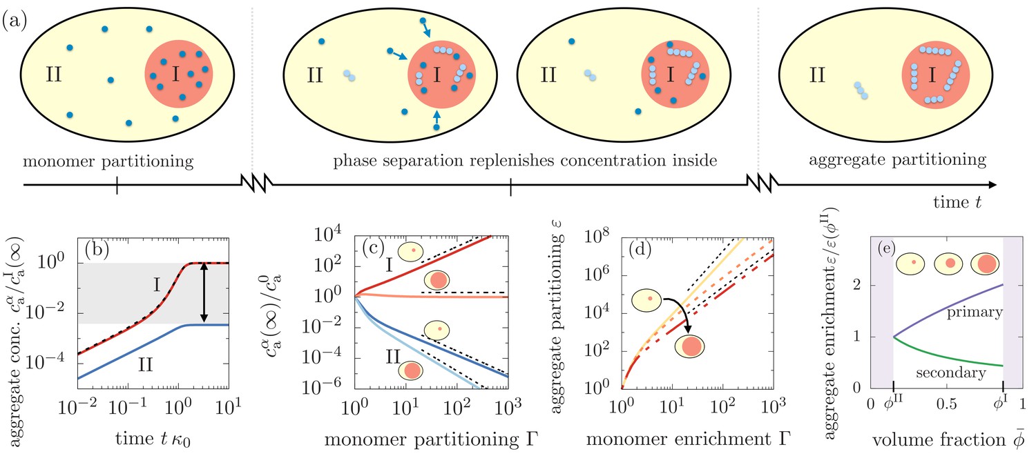
Segregation of aggregates into compartment I via positive feedback mediated by phase separation.

(a) Sketch of aggregation kinetics inside the two compartments I and II. Left: Initially, monomers get enriched on a short diffusive time scales due to the partitioning mediated by the phase separated compartments (Equation 1). Center: Monomers slowly aggregate. More aggregates nucleate and grow in compartment I due to the initial partitioning of monomers. This pronounced, initial aggregation causes a continuous monomer flux into compartment I, further promoting aggregation (positive feedback indicated by arrows). Right: Partitioning of monomers together with the positive feedback can cause a very pronounced accumulation of aggregates relative to compartment II. (b) Aggregate concentration $c_{a}^{α} (t)$ as a function of time $t$ obtained from solving numerically and analytically Equation 3 actually confirms that aggregates can enrich by several orders of magnitude. (c) The asymptotic concentrations $c_{a}^{I} (\infty)$ and $c_{a}^{I I} (\infty)$ inside each of the compartment inversely scale for small compartments, while for large compartment I, aggregate enrichment therein vanishes while depletion inside compartment II is dominated by primary nucleation. The asymptotic concentration in the absence of monomer partitioning, $Γ = 1$ , is denoted as $c_{a}^{t o t} |_{ϕ^{I} = ϕ^{I I}}$ . Dashed line are the scalings given in the the main text. Parameters: $n_{1} = n_{2} = 2$ . (d) Partitioning factor $ε$ of aggregates inside compartment I as a function of monomer partitioning $Γ$ can reach very large values. The behavior switches from secondary nucleation dominated increase at small compartment I volumes to primary dominated growth at large volumes. Dashed line are the scalings given in Equation (6). (e) The slope of the partitioning factor as a function of mean volume fraction $\bar{ϕ}$ , equivalently speaking, volume of compartment I, changes its sign when partitioning is dominated by primary ( $n_{1} = 2, n_{2} = 0$ ) or secondary nucleation ( $n_{1} = 2, n_{2} = 2$ ). Parameters: (b,e) $Γ = 3$ consistent with weak interactions.

https://doi.org/10.7554/eLife.42315.004

Figure 4

Download asset Open asset

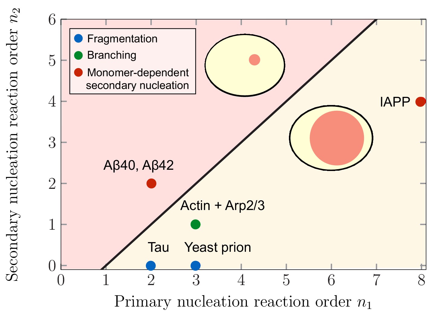
Theoretical predictions of maximal aggregate partitioning for various aggregating systems.

Our predictions are summarized by a phase diagram depicting that aggregating systems characterized by different reaction orders for primary and secondary nucleation, $n_{1}$ and $n_{2}$ , show maximal aggregate partitioning for large or small compartments, respectively. The two regions where either large or small compartments lead to a larger partitioning of aggregates is separated by the line $n_{2} = n_{1} - 1$ determined from Equation 6. For $n_{2} > n_{1} - 1$ small compartments lead to larger aggregate partitioning, while for $n_{2} < n_{1} - 1$ , larger compartments are beneficial. To illustrate which scenario might apply to which kind of aggregating system, we indicate the measured values of the primary and secondary reaction orders for a range of systems propagating through fragmentation (blue), lateral branching (green) or monomer-dependent secondary nucleation (red): Tau (Kundel et al., 2018), yeast prion Ure2p (Zhu et al., 2003), IAPP (Ruschak and Miranker, 2007), Amyloid-β40 (for monomer concentrations below 5 μM) (Meisl et al., 2014), Amyloid-β42 (Cohen et al., 2013).

https://doi.org/10.7554/eLife.42315.005

Figure 5

Download asset Open asset

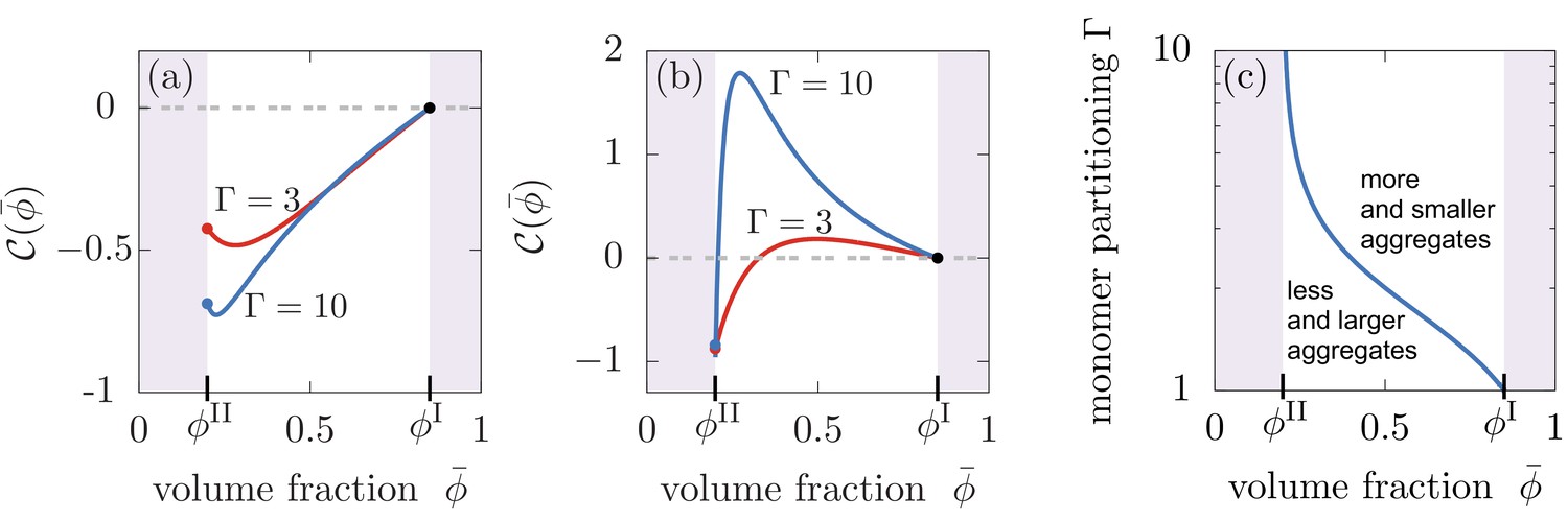
Compartments can change the total aggregate concentration compared to the homogeneous state without compartments.

(a,b) Relative asymptotic aggregate concentration $𝒞 (\bar{ϕ}, Γ) = (c_{a}^{t o t} - c_{a}^{t o t} |_{ϕ^{I} = ϕ^{I I}}) / c_{a}^{t o t} |_{ϕ^{I} = ϕ^{I I}}$ as a function of volume fraction of the compartment material $\bar{ϕ}$ (connected to compartment volume $V^{I} (\bar{ϕ}) = V (\bar{ϕ} - ϕ^{I I}) / (ϕ^{I} - ϕ^{I I})$ ), where $c_{a}^{t o t} |_{ϕ^{I} = ϕ^{I I}}$ is the concentration of the homogeneous state in the absence of compartments. (a) For secondary reaction order $n_{2} < 1$ , the total amount of aggregates is decreased compared to the case without compartments for all values of monomer partitioning $Γ$ and compartment material volume fractions $\bar{ϕ}$ and compartment volumes $V^{I}$ . (b) However, for $n_{2} > 1$ , the total amount of aggregates is either increased or decreased relative to the homogeneous state. (c) Depending on the value of the monomer partitioning $Γ$ , compartments either lead to more but shorter aggregates (large $Γ$ , larger volume controlled by $\bar{ϕ}$ ) or less but larger aggregates Parameters: (a) $n_{1} = 2$ , $n_{2} = 0$ ; (b,c) $n_{1} = 2$ , $n_{2} = 3$ .

https://doi.org/10.7554/eLife.42315.006

Appendix 3—figure 1

Download asset Open asset

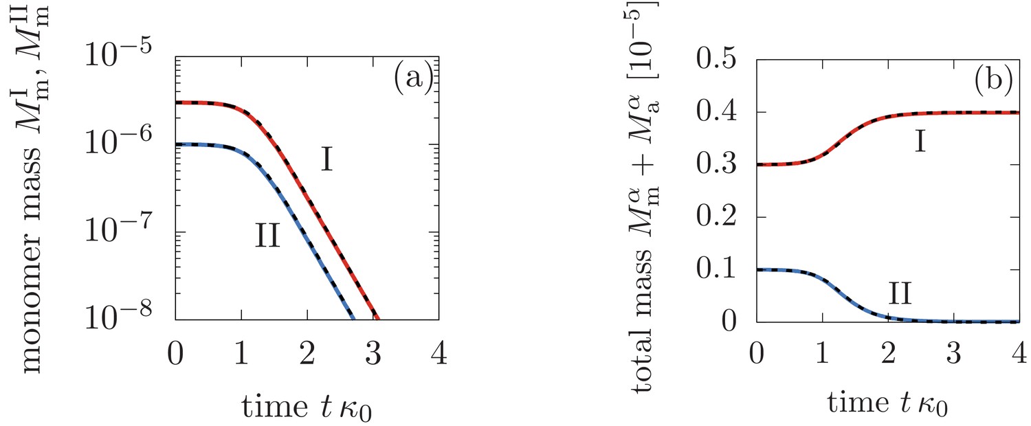
Comparison between the analytical solutions Equations (46), (47), (48) (dashed lines) and the numerical solution to Equation (3) in the main text (solid lines).

Panel (a) shows the monomer mass concentration in phase I and II, while (b) depicts the total monomer mass in form of monomers and aggregate mass in each phase. The parameters are: $k_{+} = 10^{6}$ M^-1s^-1, $k_{1} = 10^{- 4}$ M^-1s^-1, $k_{2} = 10^{4}$ M^-2s^-1, $M_{m}^{tot} = 4 μ$ M, $n_{1} = n_{2} = 2$ , $Γ = 3$ , $ξ = 1$ and $k^{α} / κ_{0} = 100$ for $α = I, I I$ .

https://doi.org/10.7554/eLife.42315.011

Additional files

Transparent reporting form: https://doi.org/10.7554/eLife.42315.007
Download elife-42315-transrepform-v1.docx

Download links

A two-part list of links to download the article, or parts of the article, in various formats.

Downloads (link to download the article as PDF)

Article PDF

Open citations (links to open the citations from this article in various online reference manager services)

Mendeley

Cite this article (links to download the citations from this article in formats compatible with various reference manager tools)

Christoph Weber
Thomas Michaels
L Mahadevan

(2019)

Spatial control of irreversible protein aggregation

eLife 8:e42315.

https://doi.org/10.7554/eLife.42315

Sign up for email alerts

Privacy notice