Figures and data in A multiphase theory for spreading microbial swarms and films

Figures
Tables
Additional files

9 figures, 3 tables and 3 additional files

Figures

Figure 1

Download asset Open asset

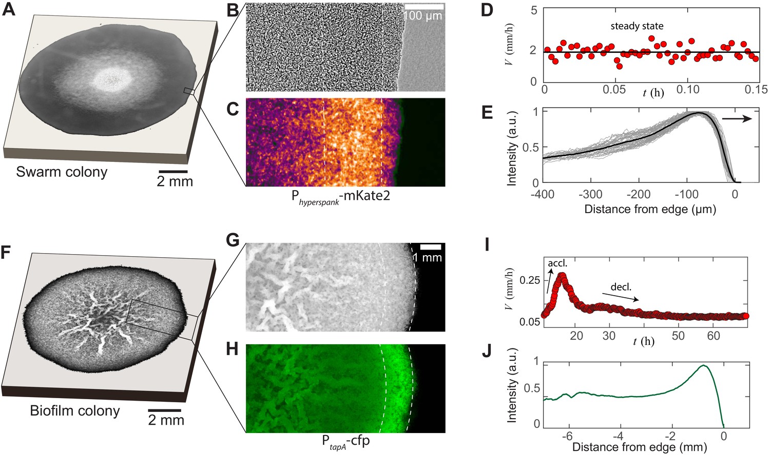
Experimental features of microbial swarms and biofilms.

(A) Snapshot of a *Bacillus subtilis* swarm expanding on a 0.5 wt% LB/agar gel. (**B,C**) Brightfield and fluorescent zoom images of the leading swarm edge of a MTC822 strain containing the fluorescent *P_hyperspank*-mKate2 reporter that is expressed constitutively. The dashed white lines indicates the extent of the multi-cellular region. (D) Expansion velocity of the swarm measured at intervals of 10 s over a 10 min period. The solid line corresponds to a mean steady-state velocity of $V$ = 2 mm/h. (E) Mean intensity traces of the constitutive fluorophore (mKate2) representing bacterial densities profiles plotted in the moving steady-state frame. The dark grey traces represent separate density profile measurements taken every 10 s in the advancing swarm. The solid line represents the density profile averaged over a period of 30 min. (F) A *Bacillus subtilis* biofilm colony developing on a 1.5 wt% MSgg/agar gel. (**G,H**) Brightfield and fluorescent zoom images of the biofilm colony formed by a MTC832 strain harboring the *P_tapA*-cfp fluorescent reporter expressed in cells synthesizing the extracellular polymeric matrix (EPS). The dashed white lines indicates the extent of an active peripheral zone signifying localized EPS production. (I) Expansion velocity of the biofilm colony measured at intervals of 10 mins over a 72 hr period. The peak expansion velocity of $V$ = 0.22 mm/h occurs at $t$ ∼ 18 h after inoculation. (J) Azimuthally averaged matrix reporter activity (cfp) as a function of spatial distance within the biofilm.

https://doi.org/10.7554/eLife.42697.003

Figure 2

Download asset Open asset

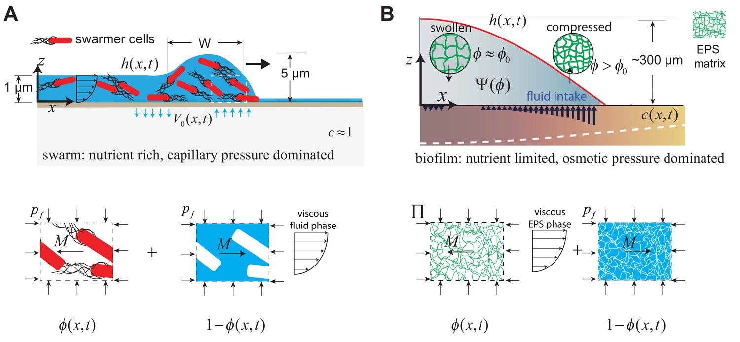
Geometry and variables governing colony expansion in (A) microbial swarms, and (B) bacterial biofilms, respectively.

In both cases, the total thickness of the microbial colony is $h (x, t)$ , the averaged nutrient concentration field is $c (x, t)$ , the volume fraction of the active phase is $ϕ (x, t)$ , the volume fraction of the fluid phase is $1 - ϕ (x, t)$ , and the fluid influx across the agar/colony interface is denoted by $V_{0} (x, t)$ . As shown on the bottom panel, the active phase constitutes swarmer cells in the microbial swarm, and secreted EPS polymer matrix in the biofilm. The pressure in the fluid phase is $p_{f}$ and the effective averaged pressure in the active phase is $Π$ . In the swarm cell phase, $Π = p_{f}$ , while the EPS phase effective pressure is $Π = p_{f} + ϕ Ψ (ϕ)$ , where $Ψ (ϕ)$ is the swelling pressure and is related to Flory-Huggins osmotic polymer stress (see Equation A28). The momentum exchange between the two phases is denoted by $M$ , which includes the sum of an interfacial drag term and an interphase term as detailed in Equation (A11) in the Appendix.

https://doi.org/10.7554/eLife.42697.005

Figure 3

Download asset Open asset

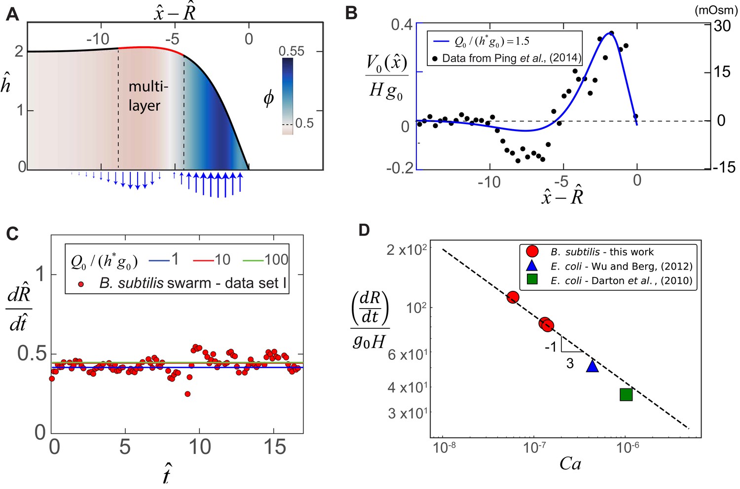
Steady-state morphology and fluid transport in a bacterial swarm obtained by solving (8) for $α_{1}$ = 0.2, $α_{2}$ = 1.5 and $ϕ_{0}$ = 0.5.

(A) Plot of the steady-state thickness $\hat{h} = h / H$ against the scaled distance $\hat{x} - \hat{R}$ , where $\hat{x} = x / (H {𝐶𝑎}^{- 1 / 3})$ and $\hat{R}$ is the radius. The solid red line indicates a region of increased thickness, and the colormap quantifies variations in $ϕ$ , the local volume fraction. (B) Plotted on the left-axis is the numerical steady-state fluid uptake profile within the swarm (solid line) calculated from Equation (4). On the right axis are experimental measurements of the steady-state osmotic pressure within an expanding *E. coli* swarm (filled circles), reproduced from Ping et al. (2014), with the baseline reference value shifted to zero, and with distances normalized by $L$ = 50 μm. (C) Predicted steady-state radial colony expansion speeds within the swarm for values of $α_{2} = Q_{0} / (H g_{0}) = 1$ , 10 and 100 respectively. The data points are expansion speeds in *B. subtilis* swarms measured over 20 min, and scaled using $U$ = 1.3 μm $s^{- 1}$ and $g_{0}$ 0.013 s^-1. (D) Comparison between the swarm expansion velocities $d R / d t$ measured for five separate colonies (see Appendix 2) and the estimated capillary number. For each experiment, $g_{0}$ was obtained by fitting the steady state solution of Equations (7) and (8) to the swarm velocity. The dashed line corresponds to the predicted scaling law in Equation (5).

https://doi.org/10.7554/eLife.42697.006

Figure 4

Download asset Open asset

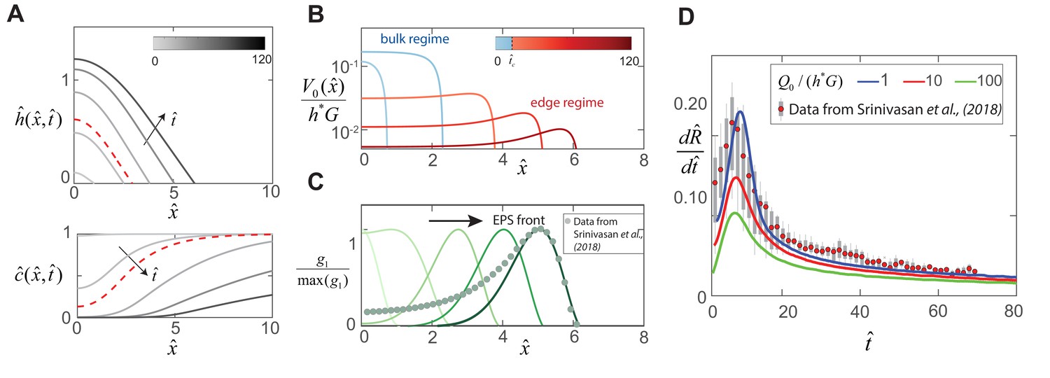
Dynamics of EPS production and biofilm expansion obtained by solving (12 - 14) with $β_{1} = 6.7$ , $β_{2} = 0.01$ , $β_{3} = 0.02$ , $β_{4} = 1$ and $β_{5} = 1.7$ .

(A) On the top are thickness profiles $\hat{h} (\hat{x}, \hat{t})$ of an expanding biofilm colony, at time intervals of $\hat{t}$ = 1, 5, 20, 50 and 90. The nutrient field $c (x, t)$ at corresponding time intervals is plotted at the bottom. The dotted red line indicates profiles at ${\hat{t}}_{c}$ = 8, the transition point between the bulk and edge expansion regimes. (B) Variation of the vertical fluid uptake profile within the swarm calculated from Equation (9). The light blue lines correspond to the bulk growth regime for $\hat{t}$ = 1, 5 while the red lines correspond to $\hat{t}$ = 20, 50 and 90 in the edge growth regime. (C) Plots of normalized EPS production activity within the biofilm, where $g_{1}$ is evaluated using the expression in Table 1. The data points are spatial measurements of *tapA* gene activity in *B. subtilis* biofilms reproduced from Srinivasan et al. (2018), with distances scaled by $L$ = 550 μm. (D) Solid lines indicate transient colony edge expansion velocities for $β_{4} = 1, 10$ and $100$ respectively, and with other parameter values fixed as listed above. The experimental data is reproduced from Srinivasan et al. (2018) and indicates median expansion velocities (filled circles), the 25th to 75th percentile velocities (filled box), and extreme values (vertical lines), where the data has been scaled by $U = 0.5 μ$ m $s^{- 1}$ and $G = 1 / 40$ min $^{- 1}$ .

https://doi.org/10.7554/eLife.42697.007

Appendix 3—figure 1

Download asset Open asset

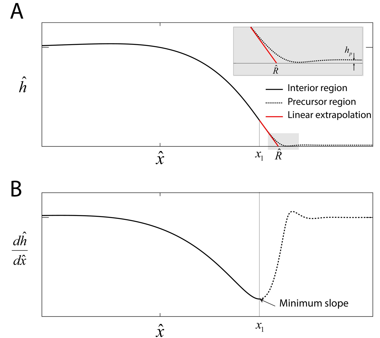
Precursor film.

(A) Numerical solution to Equations (5)-(6) in the main text that represents the swarm profile $\hat{h} (\hat{x})$ . The solid black line indicates the swarm profile in the interior region domain $\hat{x} \in [0, x_{1}]$ . The dashed line beyond $x_{1}$ denotes the precursor-film region. The solid red line represents a linear extrapolation of the swarm profile in the region $\hat{x} \in [x 1, \hat{R}]$ , where $\hat{R}$ is the swarm radius. Inset: Magnified view of the transition region, where $h_{p}$ is the precursor film of thickness. (B) The onset of the precursor film is defined at the point of the numerical profile where the slope is a minimum.

https://doi.org/10.7554/eLife.42697.016

Appendix 3—figure 2

Download asset Open asset

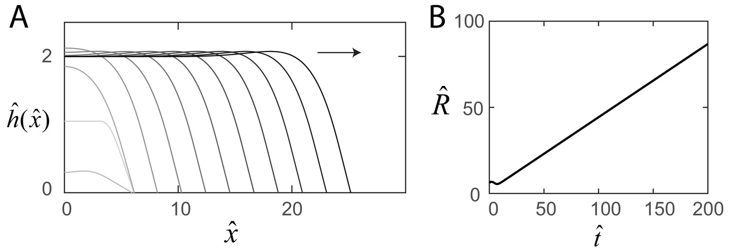
Steady-state swarm solutions.

(A) The evolution of the numerical swarm thickness $\hat{h} (\hat{x}, \hat{t})$ plotted in the laboratory frame at fixed time intervals. (B) Plot of the swarm radius as a function of time indicating steady-state solutions.

https://doi.org/10.7554/eLife.42697.017

Appendix 3—figure 3

Download asset Open asset

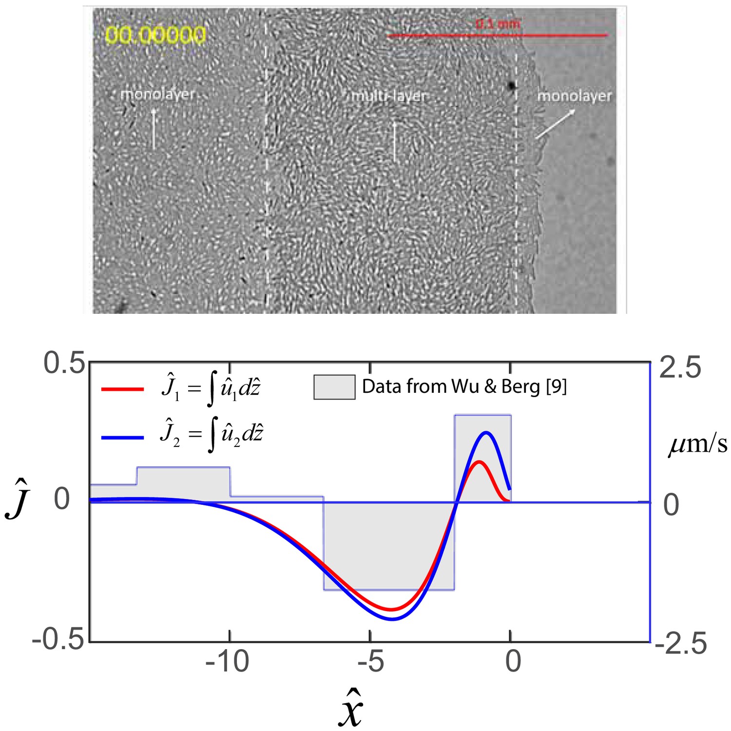
Top: Image of edge of swarm colony.

*B. subtilis* swarm colony showing the interior monolayer region, the multi-layer front, and the monolayer at the very edge of the colony. Bottom: Horizontal flows in swarms. Steady-state profile of the dimensionless net horizontal velocity $\hat{J} = \int_{0}^{\hat{h}} \hat{u} d \hat{z}$ in the swarmer cell phase (red) and fluid phase (blue). Expression for ${\hat{J}}_{1}$ and ${\hat{J}}_{2}$ are obtained from Equations (A18) and (A19) as $J_{1} = - \frac{1}{1 - ϕ} \frac{d \hat{p}}{d \hat{x}} \frac{{\hat{h}}^{3}}{3} - α_{1} \frac{d \hat{p}}{d \hat{x}} \hat{h}$ and $J_{2} = - \frac{1}{1 - ϕ} \frac{d \hat{p}}{d \hat{x}} \frac{{\hat{h}}^{3}}{3}$ , where $α_{1} = 0.2$ as discussed in the main text. The step function represents experimental flow speeds as a function of the distance form the swarm edge as measured by Wu and Berg (2012), and where the horizontal distance has been scaled by $L = 15 μ$ m.

https://doi.org/10.7554/eLife.42697.018

Appendix 3—figure 4

Download asset Open asset

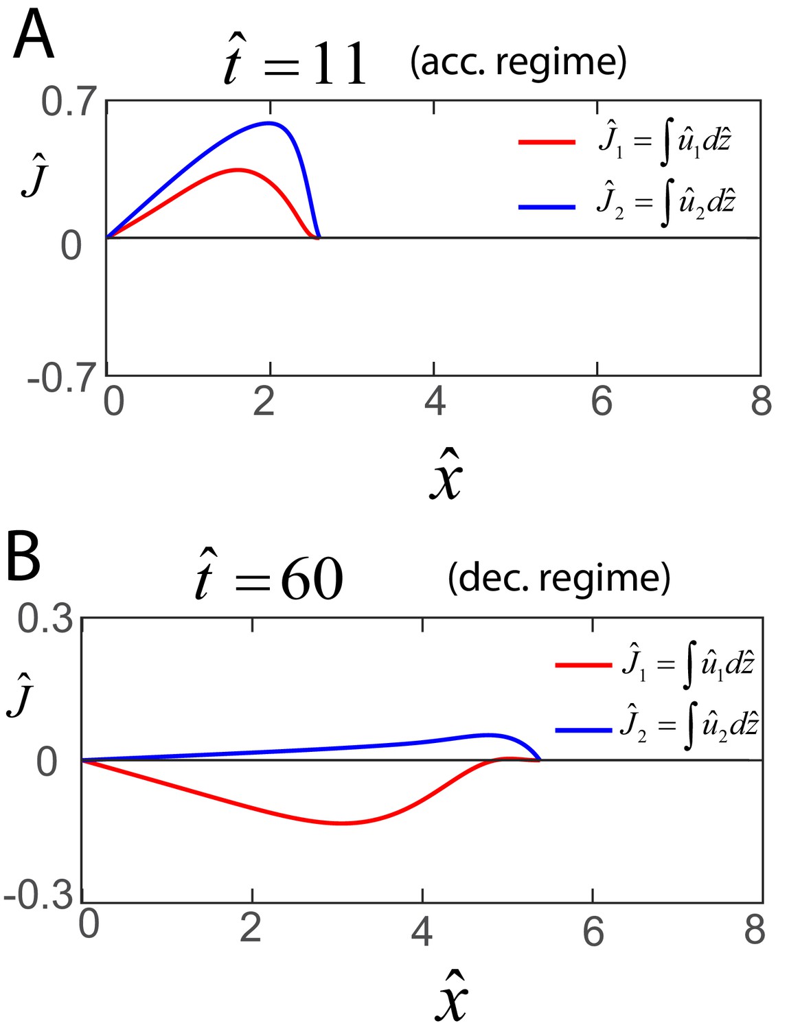
Early and late flows in biofilms.

Profile of the dimensionless net horizontal velocity $\hat{J} = \int_{0}^{\hat{h}} \hat{u} d \hat{z}$ in the EPS phase (red) and fluid phase (blue). Expression for ${\hat{J}}_{1}$ and ${\hat{J}}_{2}$ are obtained from Equations (A30) and (A31) as $J_{1} = - \frac{β_{1}}{ϕ} \frac{d \hat{Π}}{d \hat{x}} \frac{{\hat{h}}^{3}}{3}$ and $J_{2} = - \frac{β_{1}}{ϕ} \frac{d \hat{Π}}{d \hat{x}} \frac{{\hat{h}}^{3}}{3} - β_{3} \frac{1 - ϕ}{ϕ} \frac{d \hat{p}}{d \hat{x}} \hat{h}$ , where $β_{1} = 6.7$ and $β_{3} = 0.02$ as discussed in the main text.

https://doi.org/10.7554/eLife.42697.019

Appendix 3—figure 5

Download asset Open asset

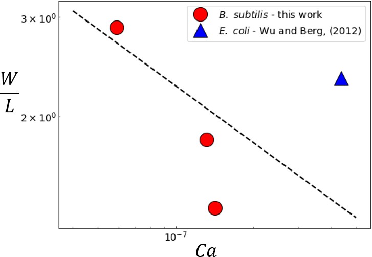
Variation of the experimentally measured multilayer swarm width $W$ with $C a$ .

For *B. subtilis* swarm experiments, the value of $W$ was determined by considering the width of the region where the mean constitutive fluorophore intensity $I > 0.7 max (I)$ (See Figure 1E). The multilater width in the *E. coli* swarm was reported as 154 μm ± 27 μm by Wu and Berg (2012). The dashed line corresponds to the predicted scaling from Equation (6).

https://doi.org/10.7554/eLife.42697.020

Tables

Table 1

Definitions of fluxes for swarms and films

Definitions of the active phase horizontal flux $Q_{1}$ , the fluid phase horizontal flux $Q_{2}$ , active phase growth term $g_{1} (h, ϕ, c)$ , osmotic influx term $V_{0} (x)$ , and nutrient consumption term $g_{2} (h, ϕ, c)$ for bacterial swarms and films in the generalized thin film evolution equations described by Equations (1–3). Here, $μ_{1}$ is the biofilm viscosity, $μ_{2}$ is the fluid viscosity, $p_{f}$ is the fluid phase pressure, $Π$ is the effective pressure in the active phase, $g_{0}$ is effective swarmer cell growth rate, $G$ is the EPS production rate, $Γ$ is the nutrient consumption rate per unit concentration, $K$ is the nutrient half-velocity constant and $d$ is the thickness of the substrate. For swarms, the active phase corresponds to the swarmer cell phase, and for biofilms, the active phase is the EPS polymer matrix.

https://doi.org/10.7554/eLife.42697.004

	Variables	Swarms	Biofilms
Flux (Phase I)	$Q_{1} (x)$	$- \frac{h^{3}}{3 μ_{2}} \frac{ϕ}{1 - ϕ} \frac{\partial p_{f}}{\partial x} - \frac{h ϕ}{ζ} \frac{\partial p_{f}}{\partial x}$	$- \frac{h^{3}}{3 μ_{1}} \frac{\partial Π}{\partial x}$
Flux (Phase II)	$Q_{2} (x)$	$- \frac{h^{3}}{3 μ_{2}} \frac{\partial p_{f}}{\partial x}$	$- \frac{h^{3}}{3 μ_{1}} \frac{1 - ϕ}{ϕ} \frac{\partial Π}{\partial x} - \frac{h}{ζ} \frac{(1 - ϕ)^{2}}{ϕ} \frac{\partial p_{f}}{\partial x}$
Osmotic influx	$V_{0} (x)$	$Q_{0} (\frac{ϕ}{1 - ϕ} - \frac{ϕ_{0}}{1 - ϕ_{0}})$	$Q_{0} (ϕ^{3} - ϕ_{0}^{3})$
Growth term	$g_{1} (h, c, ϕ)$	$g_{0} h ϕ (1 - \frac{h ϕ}{H ϕ_{0}})$	$G h ϕ \frac{c}{K + c} (1 - \frac{h ϕ}{H ϕ_{0}})$
Nutrient uptake	$g_{2} (h, c, ϕ)$	-	$\frac{Γ ϕ h}{d} \frac{c}{K + c}$

Appendix 2—table 1

List of the symbols, descriptions, and numerical value for each of the parameters used.

https://doi.org/10.7554/eLife.42697.013

Variable	Description	Numerical value
$H$	vertical length scale	swarms - 0.5 μm biofilms - 400⁢ μm ⁢
$L$	horizontal length scale	swarms - 100 ⁢μ⁢m biofilms - 1100⁢ μ⁢m
$U$	horizontal velocity scale	swarms - 1.3 ⁢μ⁢m/s biofilms - 0.5 ⁢μ⁢m/s
$ϕ_{0}$	equilibrium volume fraction of active phase	swarms - 0.5 biofilms - 0.04
$Q_{0}$	vertical fluid velocity scale	swarms - 10^–2⁢μ⁢m/s biofilms - 0.04
$g_{0}$	effective swarm cell growth rate	0.005 — 0.2 s^-1
$G$	EPS production rate	1/40 min^-1
$μ_{1}$	EPS matrix viscosity	10⁵ Pa.s
$μ_{2}$	fluid viscosity	10^–3 Pa.s
$ζ$	friction coefficient per unit cell volume	10^–2 pN/(μm s^-1)
$γ$	fluid surface tension	10^-2 N/m
$Ψ_{0}$	osmotic pressure scale	2100 Pa
Dimensionless parameters: Bacterial swarm
$α_{1}$	$\frac{γ H}{ζ L^{3} U}$	0.2
$α_{2}$	$\frac{Q_{0}}{H g_{0}}$	0.1 — 4.3
Dimensionless parameters: Bacterial biofilm
$β_{1}$	$\frac{Ψ_{0} H^{2}}{μ_{1} U L}$	6.7
$β_{2}$	$\frac{γ H^{3}}{μ_{1} U L^{3}}$	0.01
$β_{3}$	$\frac{γ H}{ζ μ_{1} L^{3}}$	0.02
$β_{4}$	$\frac{Q_{0}}{H G}$	1
$β_{5}$	$\frac{S}{G}$	2

Appendix 2—table 2

Summary of the comparision between the experimental data and model.

The experimentally measured quantities are the colony expansion speed $V = d R / d t$ and multilayer region thickness $W$ . The value of $α_{2}$ is determined by fitting Equations (7)-(8) to the expansion velocity, leading to estimates of the effective growth rate $g_{0}$ , the horizontal length scale $L$ and the capillary number $C a$ .

https://doi.org/10.7554/eLife.42697.014

No	Reference	$V = \frac{d R}{d t}$ μms^-1 (exp)	$W$ μm (exp)	$α_{2}$ (model)	$g_{0}$ s^-1 (model)	$L$ μm (model)	$C a$ × 10^-7 (model)
1	B. subtilis this work - (data set I)	0.56	178	1.49	0.013	98	1.32
2	B. subtilis this work - (data set II)	0.26	368	4.33	0.005	128	0.59
3	B. subtilis this work - (data set III)	0.60	132	1.35	0.015	96	1.42
4	E. coli Wu and Berg, 2012	1.7	154	0.30	0.07	66	4.38
5	E. coli Darnton et al., 2010	3.8	-

Additional files

Source code 1 COMSOL file that implements the numerical solutions to Equations (7)-(8) governing bacterial swarm expansion.: https://doi.org/10.7554/eLife.42697.008
Download elife-42697-code1-v1.mph
Source code 2 COMSOL file that implements the numerical solutions to Equations (12)-(14) governing bacterial biofilm expansion.: https://doi.org/10.7554/eLife.42697.009
Download elife-42697-code2-v1.mph
Transparent reporting form: https://doi.org/10.7554/eLife.42697.010
Download elife-42697-transrepform-v1.docx

Download links

A two-part list of links to download the article, or parts of the article, in various formats.

Downloads (link to download the article as PDF)

Article PDF

Open citations (links to open the citations from this article in various online reference manager services)

Mendeley

Cite this article (links to download the citations from this article in formats compatible with various reference manager tools)

Siddarth Srinivasan
C Nadir Kaplan
L Mahadevan

(2019)

A multiphase theory for spreading microbial swarms and films

eLife 8:e42697.

https://doi.org/10.7554/eLife.42697

Share this article

Cite this article

Experimental features of microbial swarms and biofilms.

Geometry and variables governing colony expansion in (A) microbial swarms, and (B) bacterial biofilms, respectively.

Steady-state morphology and fluid transport in a bacterial swarm obtained by solving (8) for α1 = 0.2, α2 = 1.5 and ϕ0 = 0.5.

Dynamics of EPS production and biofilm expansion obtained by solving (12 - 14) with β1=6.7, β2=0.01, β3=0.02, β4=1 and β5=1.7.

Precursor film.

Steady-state swarm solutions.

Top: Image of edge of swarm colony.

Early and late flows in biofilms.

Variation of the experimentally measured multilayer swarm width W with Ca.

Definitions of fluxes for swarms and films

List of the symbols, descriptions, and numerical value for each of the parameters used.

Summary of the comparision between the experimental data and model.

Source code 1

Source code 2

Transparent reporting form

Downloads (link to download the article as PDF)

Open citations (links to open the citations from this article in various online reference manager services)

Cite this article (links to download the citations from this article in formats compatible with various reference manager tools)

Steady-state morphology and fluid transport in a bacterial swarm obtained by solving (8) for $α_{1}$ = 0.2, $α_{2}$ = 1.5 and $ϕ_{0}$ = 0.5.

Dynamics of EPS production and biofilm expansion obtained by solving (12 - 14) with $β_{1} = 6.7$ , $β_{2} = 0.01$ , $β_{3} = 0.02$ , $β_{4} = 1$ and $β_{5} = 1.7$ .

Variation of the experimentally measured multilayer swarm width $W$ with $C a$ .