Electron cryo-tomography provides insight into procentriole architecture and assembly mechanism
- University of California, San Francisco, United States
- Centro Nacional de Biotecnologia (CSIC), Spain
- Howard Hughes Medical Institute, University of California, San Francisco, United States
Figures
Figure 1 with 2 supplements
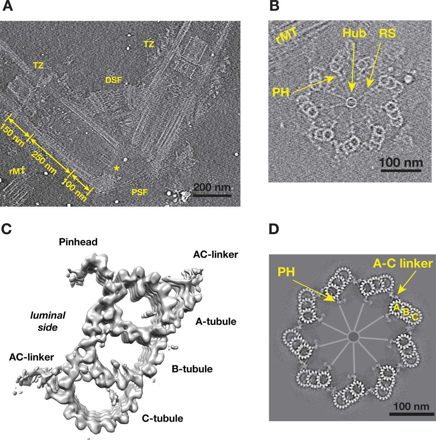
Tomographic Reconstruction and Subtomogram Averaging of the MT Triplet in Centriole and Procentriole.
(A) A slice from the reconstructed tomogram showing a pair of mother centrioles, also known as basal bodies. The central hub as part of the cartwheel is marked by a yellow asterisk. The centriole is partitioned longitudinally into three regions. The procentriole region spans 100 nm at the proximal end of the mother centriole. The central core region spans 250 nm. The distal region spans 150 nm where the triplets become doublets before reaching the transition zone (TZ). PSF: proximal striated fibers; DSF: distal striated fibers; rMT: rootlet MT. (B) A slice from the reconstructed tomogram of procentriole attached to the mother centriole via the rootlet MT. The central hub, radial spokes and pinheads are clearly visible, as well as protofilaments in some MT triplets. RS: radial spoke; PH: pinhead; rMT: rootlet MT. (C) Subtomogram average of the MT triplet from both the proximal region of mother centrioles and the procentrioles. (D) A model of procentriole viewed from its distal end. The model is generated by docking the subtomograms average in (C) into the tomogram volume in (B). The A- B- and C-tubules and the A-C linker are labeled. The central hub and the radial spokes are depicted schematically. PH: pinhead.
Figure 1—figure supplement 1
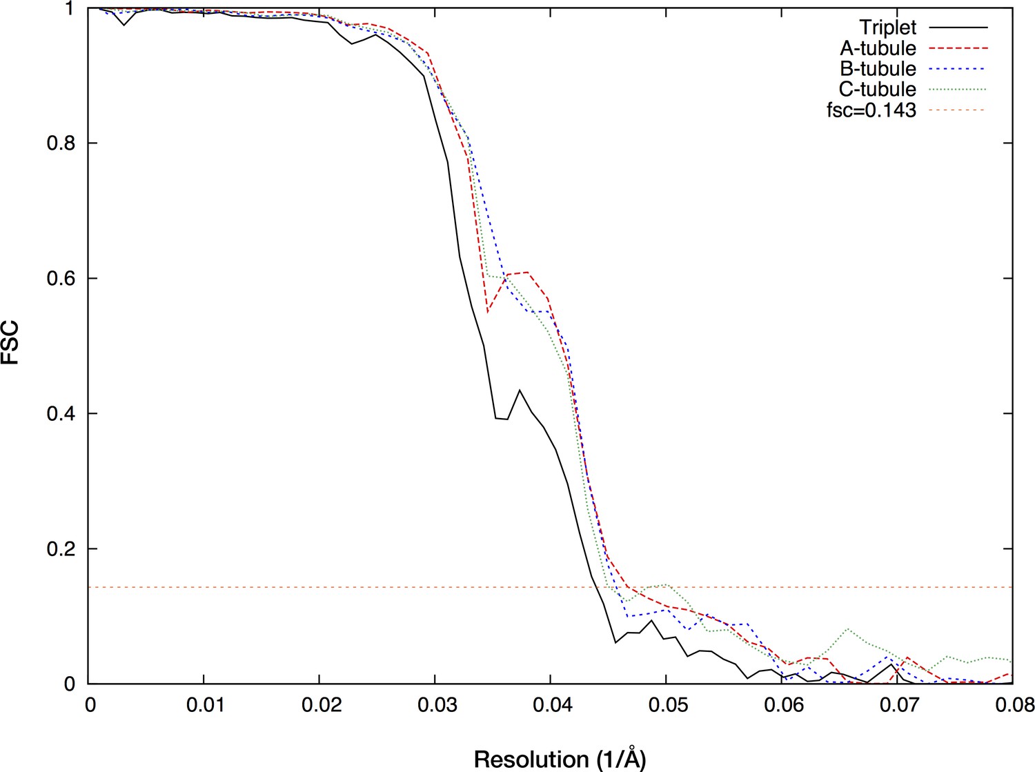
Assessing the Resolutions of Subtomogram Average by Fourier Shell Correlation (FSC) Method.
FSC curves are for the MT triplet (black, 23.0 Å), the A-tubule (red, 21.4 Å), the B-tubule (blue, 22.2 Å) and the C-tubule (green, 22.2 Å). All resolution assessments are carried out in a ‘gold-standard’ Scheme using FSC 0.143 criterion.
Figure 1—figure supplement 2
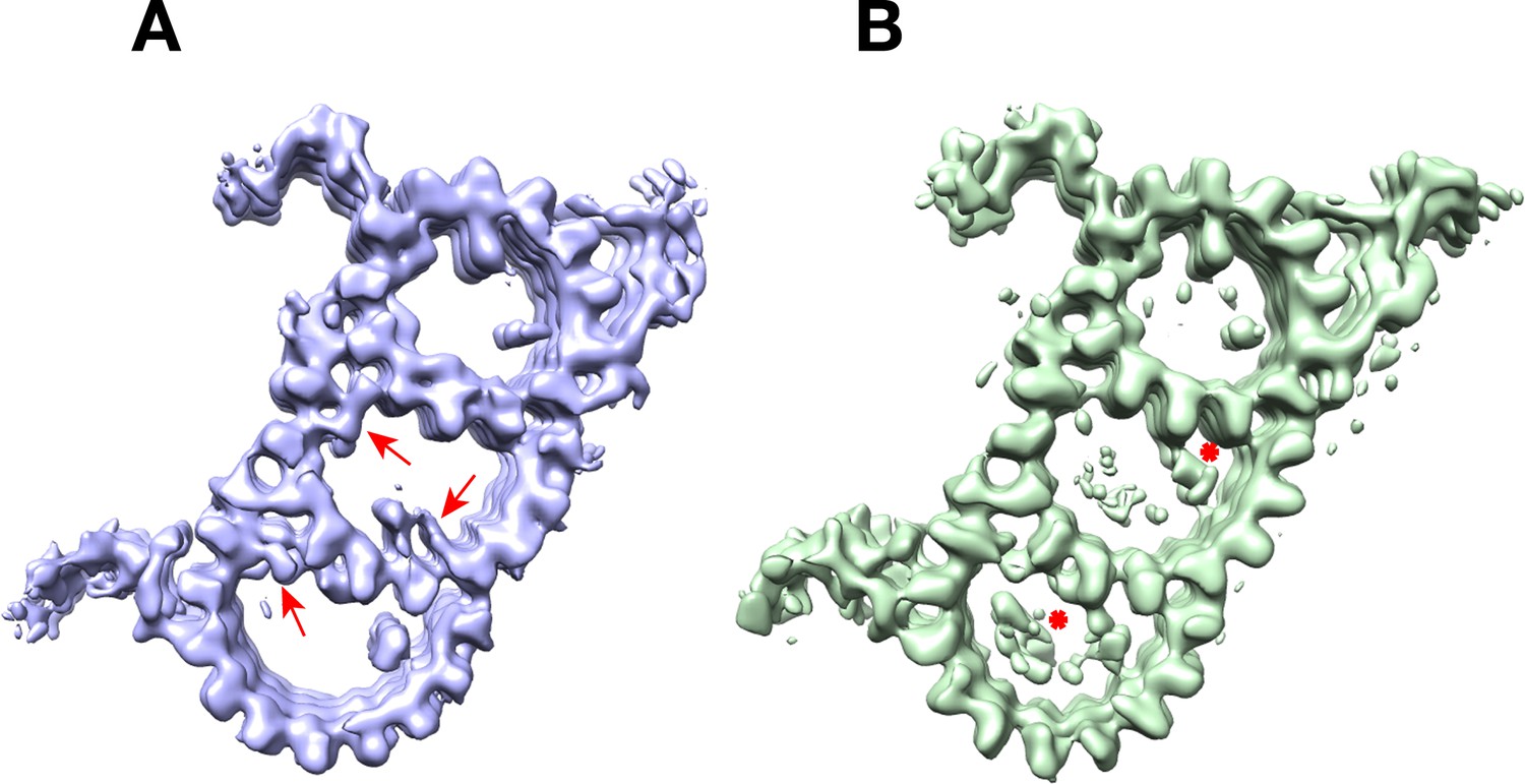
Comparing Subtomogram Averages from a Subset of Data.
(A) The triplet in blue on left is an average based on 10854 subtomograms from the proximal end of mother centrioles. (B) The triplet in light green on right is an average based on 2083 subtomograms from the 110 procentrioles that remain attached to the mother centrioles. The differences between these two structures are indicated by red arrows and by red asterisks, respectively.
Figure 2 with 14 supplements

Identifying Non-tubulin Components in Procentriole MT Triplet.
(A) The A-tubule structure. A model of 13-pf MT (red) are docked into the subtomogram average of the A-tubule. 4 MIPs identified on the A-tubule are highlighted in colors. (B) The B-tubule structure. A model of 10-pf MT (blue) are docked into the subtomogram average of the B-tubule. 4 MIPs identified on the B-tubule are highlighted in colors. (C) The C-tubule structure. A model of 10-pf MT (green) are docked into the subtomogram average of the C-tubule. 3 MIPs found at the B-C inner junction are highlighted in colors. (D) Subtomogram averaging of the pinhead structure. The pinhead is highlighted in pink color. Two dashed arrows indicate viewing directions for two images in the side view on the right. The arrows indicate PinB, PinF1 and PinF2, respectively. The arrowheads mark the tip of PinB.
Figure 2—figure supplement 1

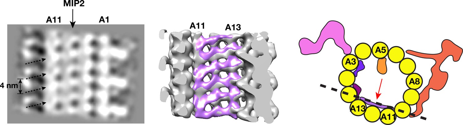
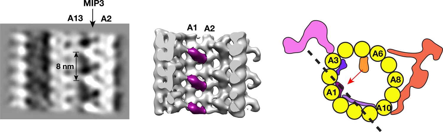
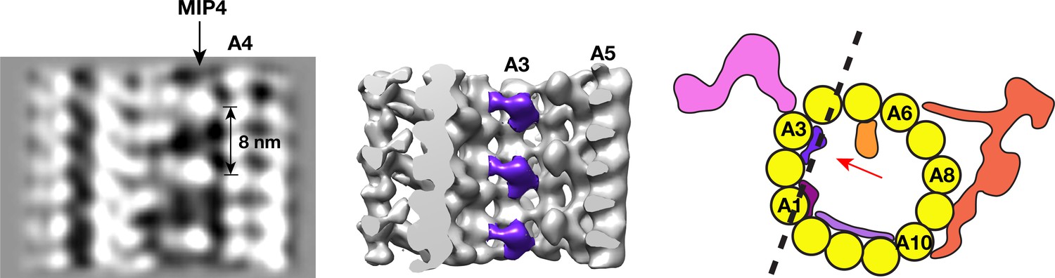
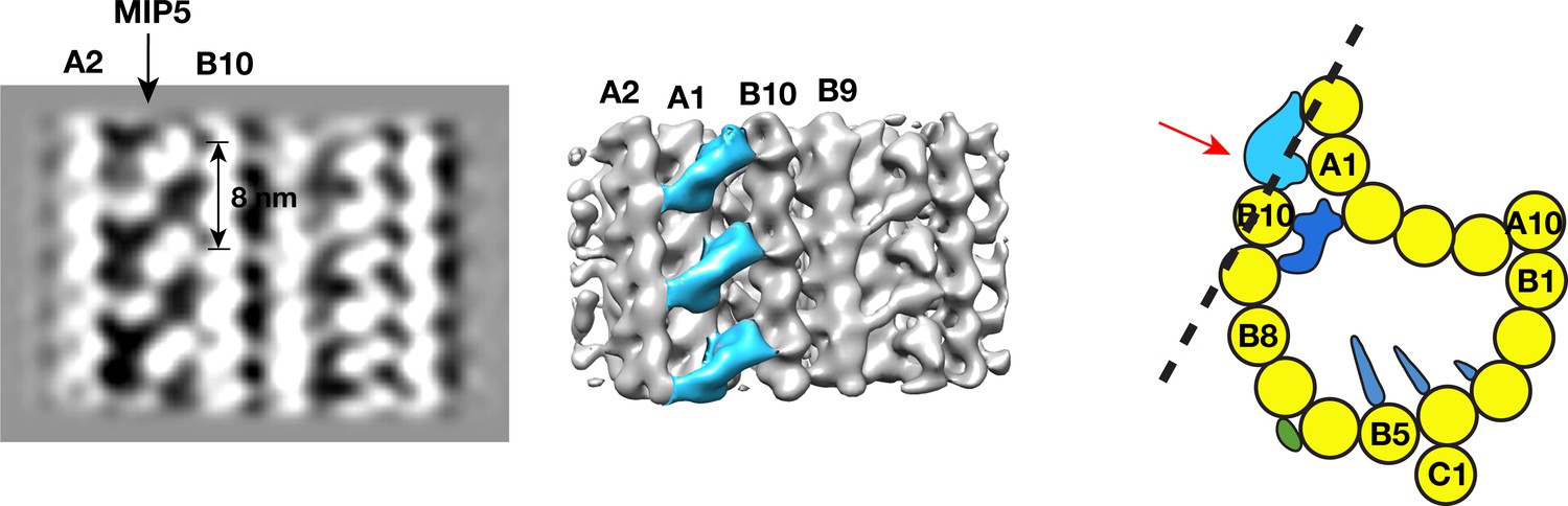
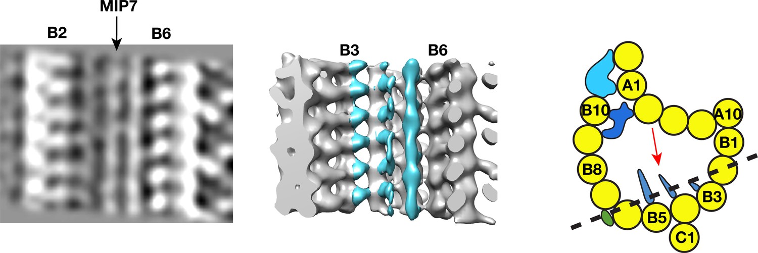
The non-tubulin Procentriole Components Associated with the MT Triplet.
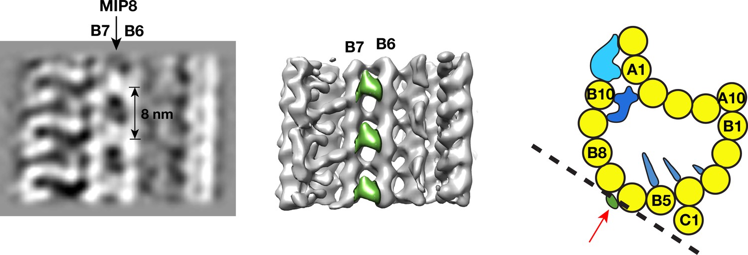
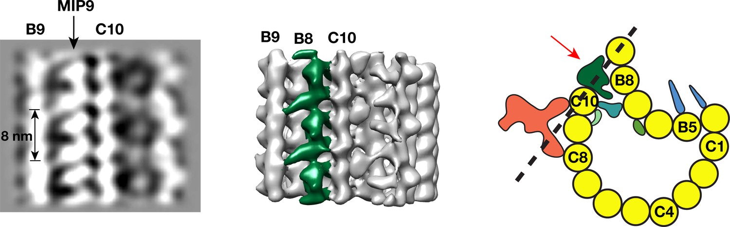
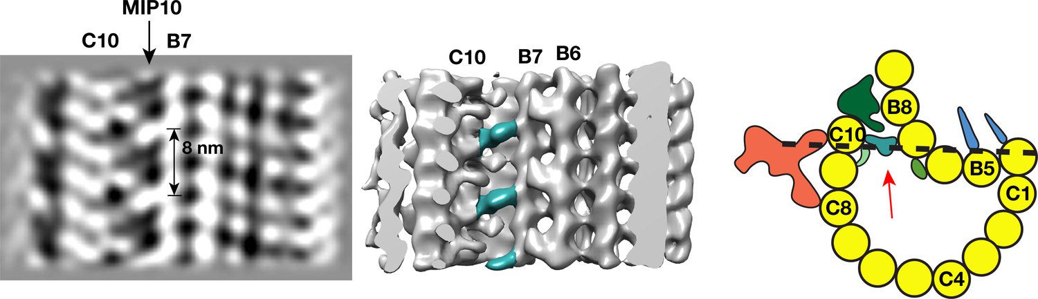
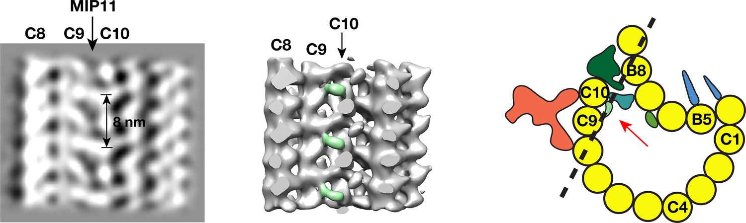
The figures show the binding pattern of 11 MIPs and their periodicity along the MT wall. In each figure, image on the left is a longitudinal cross section of the average of corresponding tubule. The middle image is a surface-rendered map with the structure of corresponding MIP highlighted in color. Image on the right is a cartoon model of the tubule. The dashed line indicates the location where the cross section goes through. The red arrow indicates viewing direction of the structure shown in the middle image. They are also summarized in Table 1.
Figure 2—figure supplement 2
The non-tubulin Procentriole Components Associated with the MT Triplet.
https://doi.org/10.7554/eLife.43434.008
Figure 2—figure supplement 3
The non-tubulin Procentriole Components Associated with the MT triplet.
https://doi.org/10.7554/eLife.43434.009
Figure 2—figure supplement 4
The non-tubulin Procentriole Components Associated with the MT Triplet.
https://doi.org/10.7554/eLife.43434.010
Figure 2—figure supplement 5
The non-tubulin Procentriole Components Associated with the MT Triplet.
https://doi.org/10.7554/eLife.43434.011
Figure 2—figure supplement 6

The non-tubulin Procentriole Components Associated with the MT Triplet.
https://doi.org/10.7554/eLife.43434.012
Figure 2—figure supplement 7
The non-tubulin Procentriole Components Associated with the MT Triplet.
https://doi.org/10.7554/eLife.43434.013
Figure 2—figure supplement 8
The non-tubulin Procentriole Components Associated with the MT Triplet.
https://doi.org/10.7554/eLife.43434.014
Figure 2—figure supplement 9
The non-tubulin Procentriole Components Associated with the MT Triplet.
https://doi.org/10.7554/eLife.43434.015
Figure 2—figure supplement 10
The non-tubulin Procentriole Components Associated with the MT Triplet.
https://doi.org/10.7554/eLife.43434.016
Figure 2—figure supplement 11
The non-tubulin Procentriole Components Associated with the MT Triplet.
https://doi.org/10.7554/eLife.43434.017
Figure 2—figure supplement 12
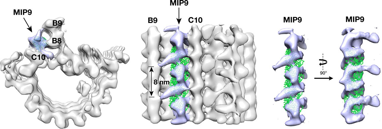
MIP9 forms a non-tubulin filament at the inner junction of B- and C-tubule.
The MIP9 density is highlighted in blue. A model of MT protofilament in green is fit into the MIP9 density. On the right panel, only the MIP9 filament is shown in two orthogonal views, the rest triplet structure is removed for clarity. The MIP9 density differs substantially from a canonical MT protofilament.
Figure 2—figure supplement 13
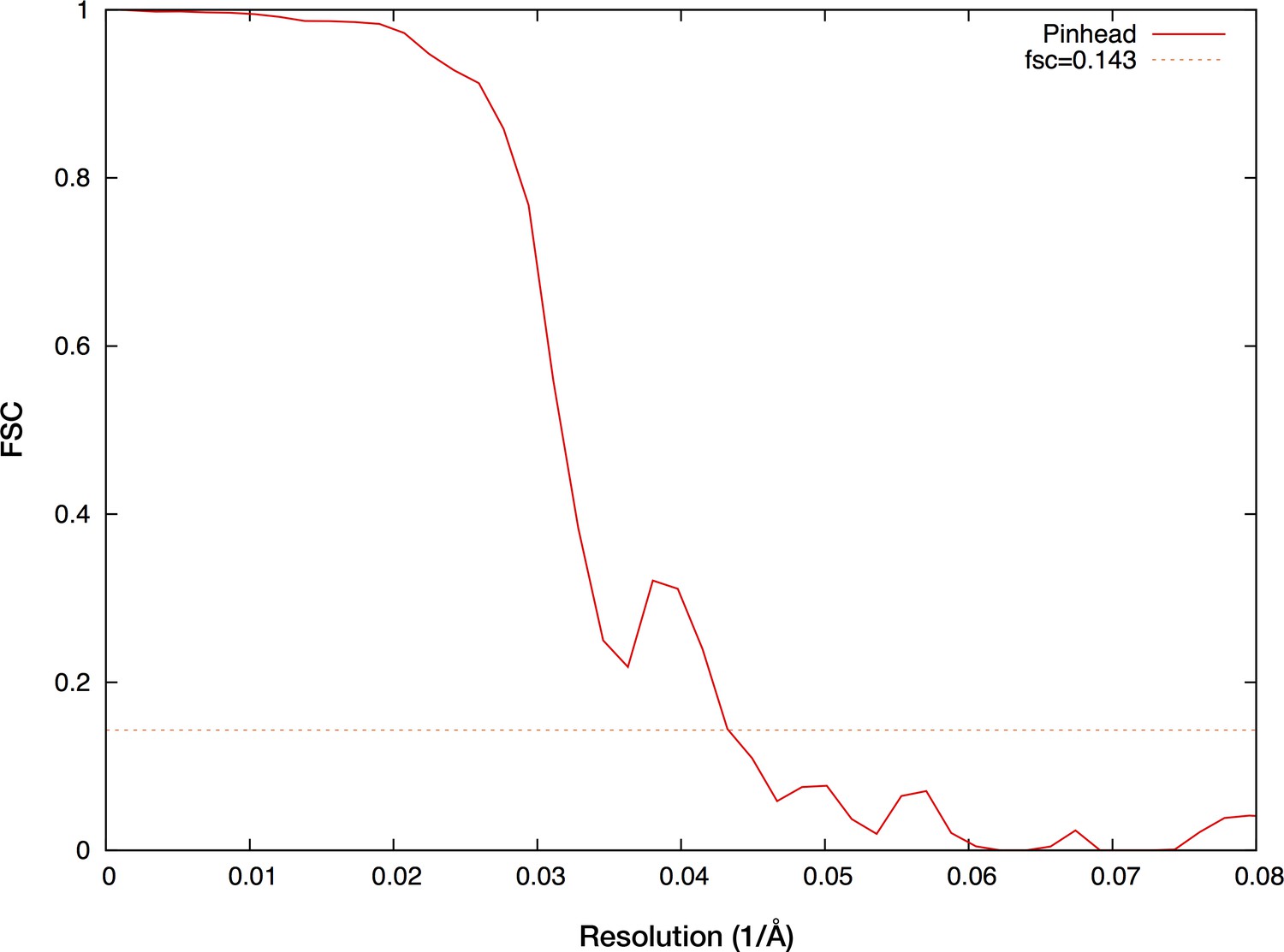
FSC curve for the averaged pinhead structure after classification (resolution: 23.1 Å).
https://doi.org/10.7554/eLife.43434.020
Figure 2—figure supplement 14

The anisotropic resolution in the pinhead structure.
The distal tip of PinB is flexible exhibiting the lowest resolution in the average (arrowhead). The local resolution is estimated by blocres in Bsoft.
Figure 3 with 6 supplements
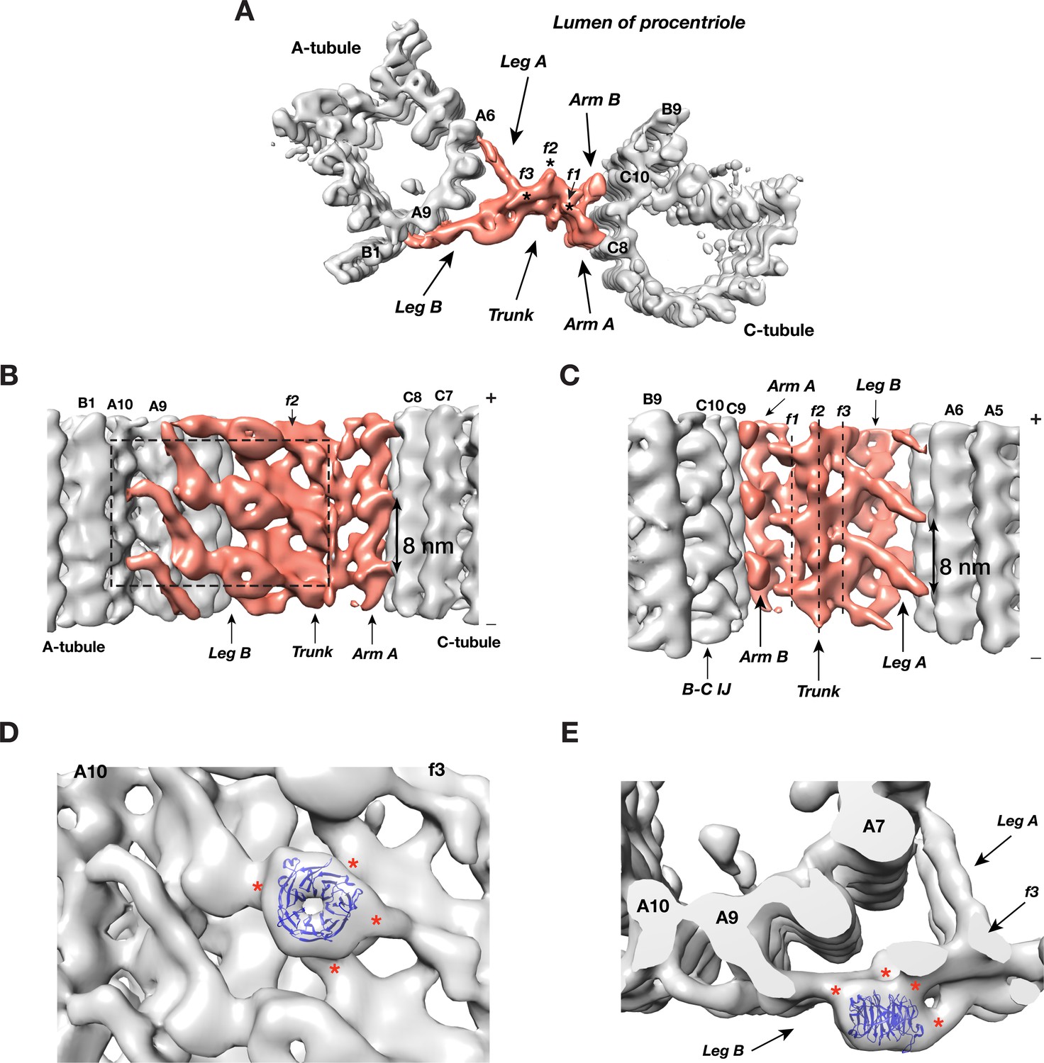
The Structure of A-C Linker.
(A) A top view of the A-C linker structure with its linked A- and C-tubules. The A-C linker is highlighted in red. Three filamental structures f1, f2 and f3 making up the central trunk running in longitudinal direction are marked with *. (B) The A-C linker viewed from outside of procentriole. The dashed square highlights the area that will be viewed in (D). (C) The A-C linker viewed from the luminal side of procentriole. Three filaments f1, f2 and f3 that make up the central trunk are marked with vertical dashed lines. They are interconnected and form a spiral. (D and E) Close up views of the Leg B in the A-C linker show a possible location of POC1. (D) is in side view from outside of the procentriole. (E) is in top view from the distal end of the procentriole. An atomic model of WD40 β-propeller domain (PDB ID 1S4U) is fitted into the doughnut-shaped density in Leg B. The red * indicate connecting points of this WD40 domain to the rest of Leg B structure and to the f3 in central trunk.
Figure 3—figure supplement 1

Schematic diagram shows the classification process for identifying intact A-C linker associated with the A-tubule.
The number of subtomogram in each class and the four classes identified with intact A-C linker are indicated. Total 3992 subtomograms from four classes are identified with relative intact A-C linker. Among them, 2917 (73.1%) are from the proximal end of mother centrioles. 1075 (26.9%) are from the procentrioles.
Figure 3—figure supplement 2
Subtomogram average of the A-tubule with associated A-C linker.
This is based on 3992 subtomograms (Class 1–4) identified in classification scheme in Figure 3—figure supplement 1.
Figure 3—figure supplement 3
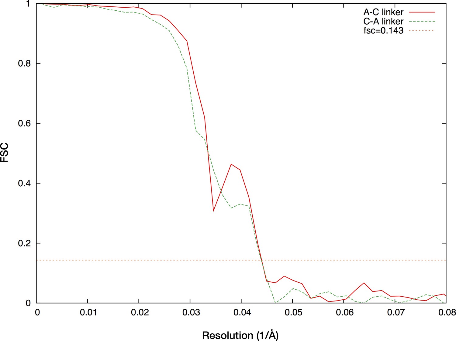
FSC curves for the averaged A-tubule and the C-tubule with more intact A-C linker after classification.
The A-tubule with associated A-C linker (red, 23.1 Å), the C-tubule with associated A-C linker (green, 23.1 Å).
Figure 3—figure supplement 4
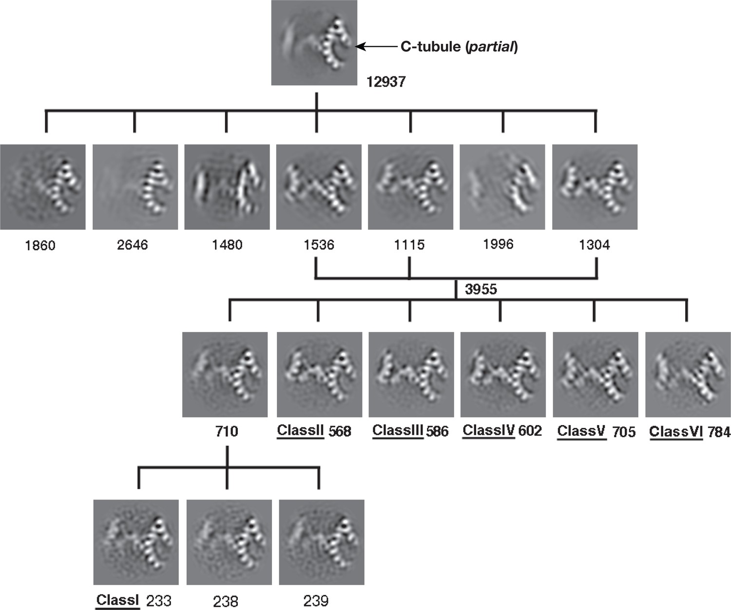
Schematic diagram showing classification process for identifying intact A-C linker associated with the C-tubule.
The number of subtomogram in each class and the six classes identified with relative intact A-C linker are indicated. The Class one is not used for further refinement and average due to its low quality. Total 3478 subtomograms from six classes are identified with relative intact A-C linker. Among them, 2611 (75.1%) are from the proximal end of mother centrioles. 867 (24.9%) are from the procentrioles.
Figure 3—figure supplement 5
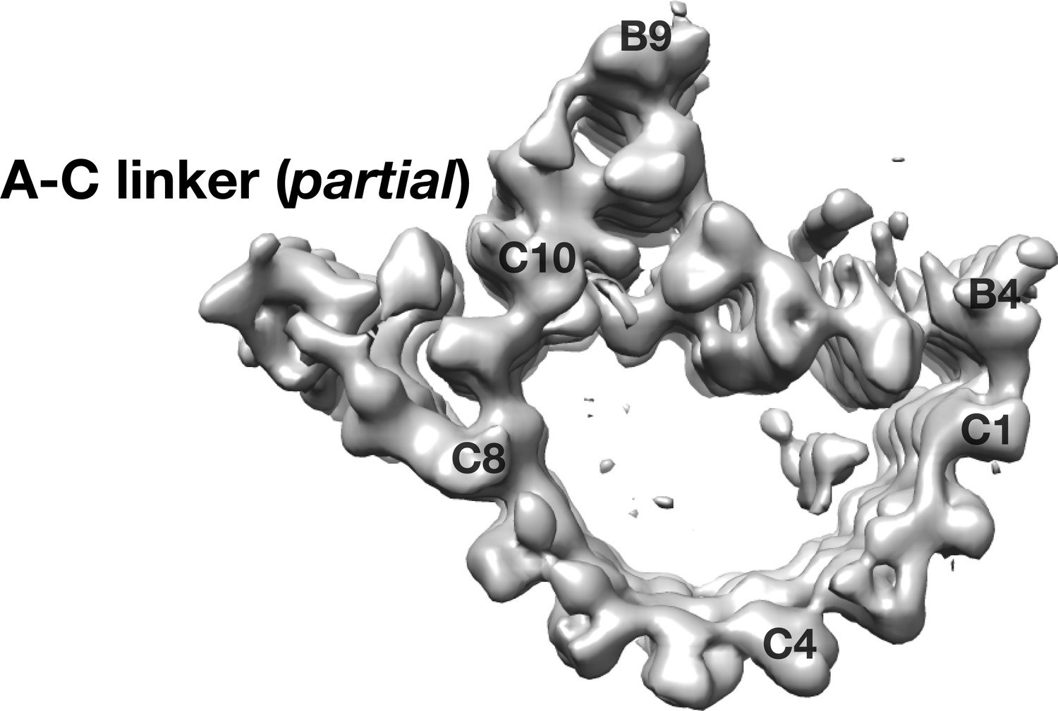
Subtomogram average of the C-tubule with associated A-C linker.
This is based on 3245 subtomograms (Class 2–6) identified in classification scheme in Figure 3—figure supplement 4.
Figure 3—figure supplement 6
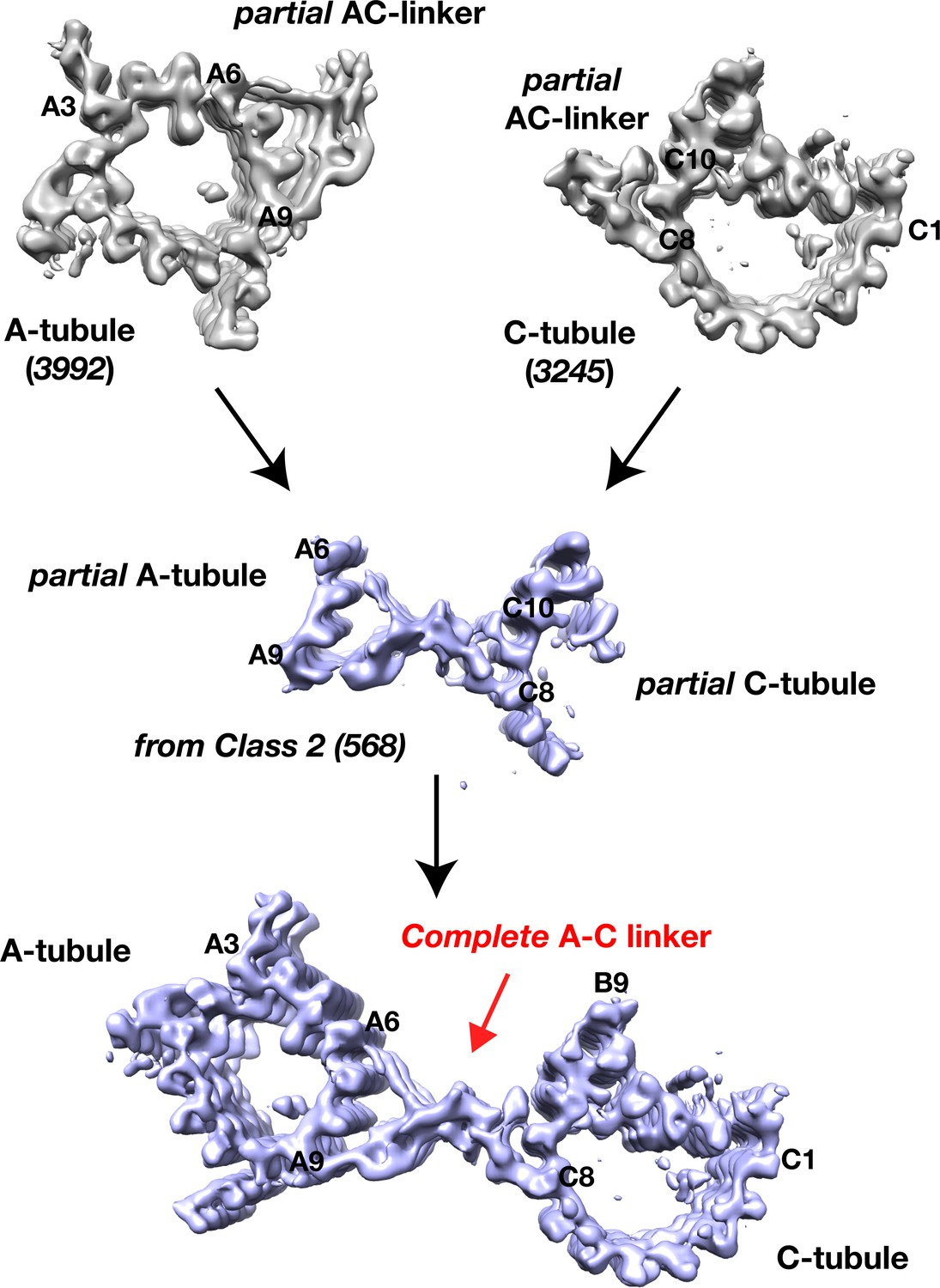
The scheme for Reconstruction of Full A-C Linker Structure.
By using this scheme, based on the 4 and 6 classes identified (illustrated in Figure 3—figure supplements 1,4), total 10 structures with full A-C linker are reconstructed showing different degrees of the twist motion. The Class 2 (568 subtomograms) identified in the second classification scheme (Figure 3—figure supplement 4) is used as an example shown in Figure 3.
Figure 4
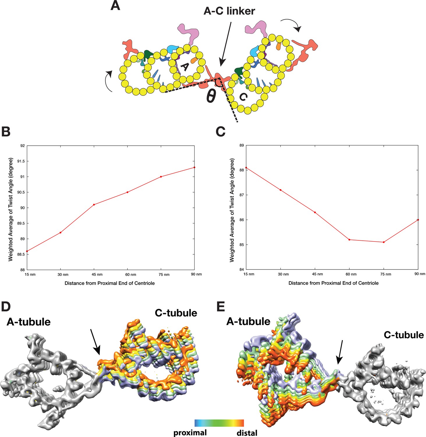
The Twist of A-C Linker Drives Procentriole Triplets in Iris Diaphragm Motion.
(A) Schematic diagram of two triplets connected by the A-C linker. θ is defined as the angle between the Arm A and the Leg B. The results of mapping and angle measurement as shown in (B-C, Table 2) are consistent with a twisting motion of two triplets as indicated by two curved arrows when moving longitudinally from proximal to distal direction. The pivot point of this twist is at the A-C linker as indicated by an arrow. (B and C) Weighted averages of twist angle along the triplet wall in two classification schemes shown in Figure 3—figure supplements 1,4. Six points along 90 nm longitudinal length of centriole are sampled starting from the proximal end. The weighted average of twist angle T at point i is defined as: Ti = ∑ θj*Nij / ∑ Nij . Nij: number of subtomogram belong to class j at point i. θj: twist angle as defined in (A) for class j. (D and E) Overlay of two sets A-C linker structure based on two classification schemes (Figure 3—figure supplements 1,4). Based on its longitudinal position, each structure is colored following a ‘heat map’ scheme. Arrows point to the pivot point, the central trunk.
Figure 5 with 1 supplement
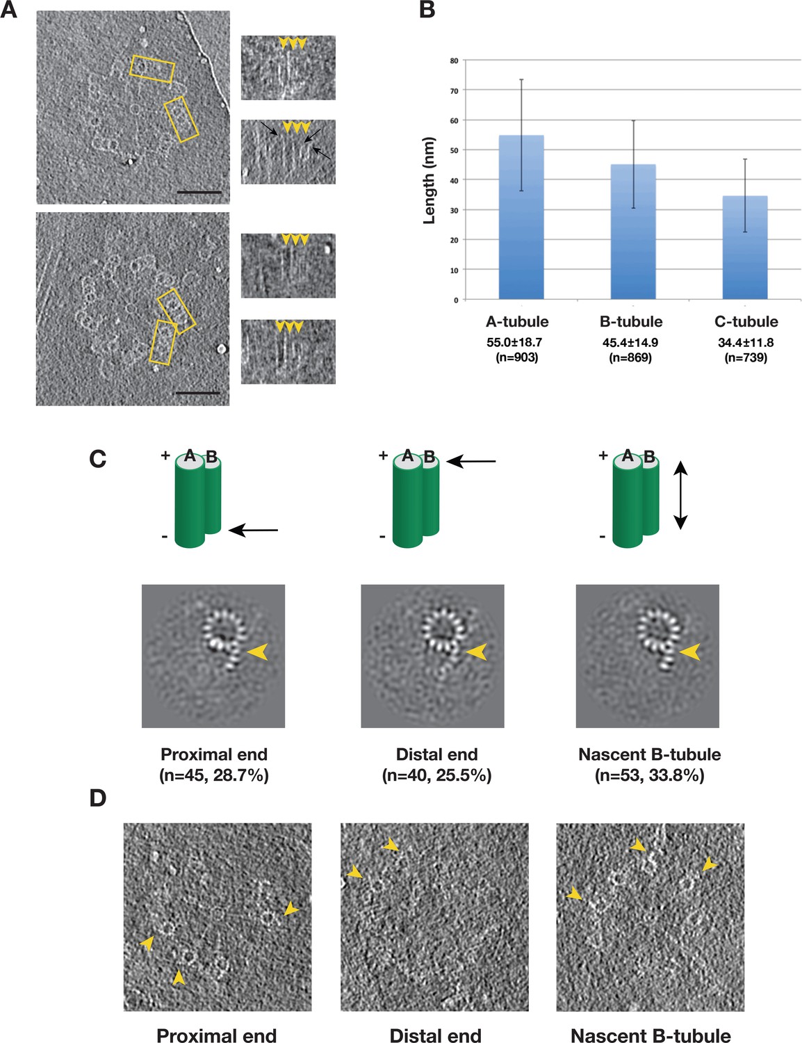
Variation of the Tubule Length in Procentriole Triplets and Detecting the B-tubule Intermediate.
(A) Two examples of procentriole in tomogram. In each, two triplets marked by yellow rectangle box are selected to depict tubule length variation as shown on the right in the longitudinal view. The distal end of each tubule is indicated by an arrowhead. Black arrows indicate examples of the slightly flared morphology at the growing end of the tubule. Scale bar: 100 nm. (B) Histogram showing length distribution for A-, B- and C-tubules. For each tubule, the average length, its standard deviation and the number of measurement are indicated. (C) The averages of incomplete B-tubule from the proximal, distal and nascent doublet, respectively. Each image is a z-projection of doublet of 9.6 nm long. The numbers of subtomogram in each class and their percentages are indicated. The arrowhead indicates PF B1. (D) Examples of incomplete B-tubule in procentriole tomogram from three classes. The incomplete B-tubules are marked by yellow arrowheads.
Figure 5—figure supplement 1
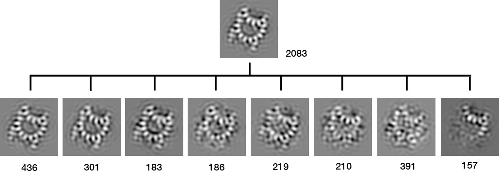
Classification and Identification of Partially Assembled B-tubule.
Total 157 subtomograms with incomplete doublet are identified as the result of classification. Images displayed are the central z-sections from the average of each class. The number of subtomogram in each class is indicated.
Figure 6 with 1 supplement
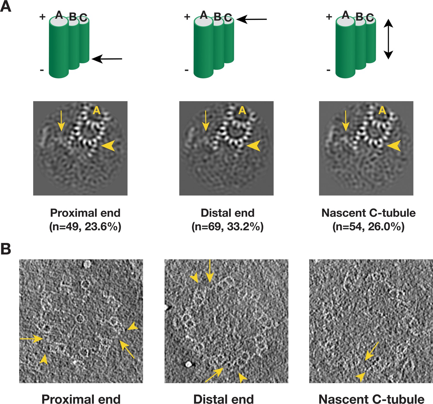
Detecting the C-tubule Intermediate.
(A) The averages of subset of subtomogram with incomplete triplet at proximal, distal end and from nascent triplet. The images are z-projection of the average where the triplet length is 9.6 nm. The numbers of subtomogram in each class and their percentages are indicated. The arrowhead points to PF C1. The arrow points to the A-C linker. (B) Examples of incomplete C-tubule in procentriole tomogram in three classes. The incomplete C-tubules are marked by yellow arrowheads. The A-C linkers are marked by yellow arrows.
Figure 6—figure supplement 1

Classification and Identification of Partially Assembled C-tubule.
Total 208 subtomograms with incomplete triplet are identified as the result of classification. Images displayed are the central z-sections from the average of each class. The number of subtomogram in each class is indicated.
Figure 7
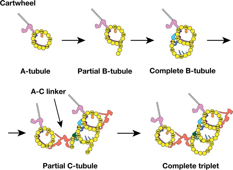
A Model for the MT Triplet Assembly in Procentriole.
In the model, the triplet assembly can be divided into five sequential steps: 1) A-tubule emerges and anchors to the pinhead in the cartwheel. It continues to elongate longitudinally. 2) B-tubule branches out at PF A10 in outer A-B junction. 3) B-tubule expands laterally from outer A-B junction toward the luminal inner A-B junction where it completes the B-tubule. 4) C-tubule branches out at both inner and outer B-C junctions. Meanwhile, the A-C linker is established. 5) The bi-directional lateral expansion of C-tubule completes the triplet assembly at this longitudinal position.
Videos
Video 1
An Aligned Tomography Tilt Series of NFAp Showing a Pair of Mother Centriole and the Attached Procentrioles.
https://doi.org/10.7554/eLife.43434.005
Video 2
Surface Rendered Structure of the A-C Linker.
https://doi.org/10.7554/eLife.43434.028
Video 3
Swing Motion of the A-C Linker and its Linked C-tubule.
The A-tubule on the left is static and is used as a reference point to show the motion.
Video 4
Swing Motion of the A-C Linker and its Linked A-tubule.
The C-tubule on the right is static and is used as a reference point to show the motion.
Video 5
An Iris-Diaphragm Motion of the Procentriole Triplets.
A longitudinal segment of the procentriole is generated by putting the averaged triplet structure back into one of the procentriole tomograms. The movie is displayed as moving through the longitudinal direction from the proximal to the distal end then backwards. The triplets twist progressively along the procentriole in a left-handed chirality with the thumb pointing towards the distal end. Two yellow arrows mark the two A-C linkers. They appear at the distal end of the longitudinal segment.
Tables
Table 1
Estimated Molecular Weight of MIPs associated with Triple.
https://doi.org/10.7554/eLife.43434.040| Name | Estimated MW (KD) | Periodicity | Location |
|---|---|---|---|
| MIP1 | 45 | 8 nm | cone-like structure associated with the lumen side of A5 |
| MIP2 | n/a | 4 nm | trellis-like structure spanning laterally from A11 to A13 |
| MIP3 | 24 | 8 nm | laterally link A13, A1 and A2 in the lumen of A-tubule |
| MIP4 | 28 | 8 nm | laterally link A2 and A3 in the lumen of A-tubule |
| MIP5 | 74 | 8 nm | inner junction of A, B-tubule, laterally link A1, A2 and B10 |
| MIP6 | 27 | 8 nm | inner junction of A, B-tubule, laterally link A1, A13, B9, B10 |
| MIP7 | n/a | 8 nm | fin-like filamental structures running longitudinally along B5, B4 B3 in the lumen of B-tubule |
| MIP8 | 15 | 8 nm | outside of B-tubule but in the lumen of C-tubule, laterally link B6 and B7 |
| MIP9 | 92 | 8 nm | inner junction of B, C-tubule, link B8, B9 and C10 |
| MIP10 | 19 | 8 nm | inner junction of B, C-tubule, link B7 and C10 |
| MIP11 | 6 | 8 nm | laterally crosslink C9 and C10 in the lumen of C-tubule |
-
Protein density = 0.849 Dalton/Å3
Yellow: MIPs associated with the A-tubule of triplet
-
Blue: MIPs associated with the B-tubule of triplet
Green: MIPs associated with the C-tubule of triplet
Table 2
Quantitive Analysis on the Twist Motion of the A-C Linker.
https://doi.org/10.7554/eLife.43434.030| A. Measurement of Twist Angle at A-C Linker | |
|---|---|
| Class | θ angle (degree) |
| I | 93 |
| II | 90 |
| III | 87 |
| IV | 83 |
| B. Measurement of Twist Angle at A-C Linker | |
|---|---|
| Class | θ angle (degree) |
| I | 96 |
| II | 93 |
| III | 90 |
| IV | 89 |
| V | 84 |
| VI | 80 |
-
A. The assignment for each class is following convention defined in Figure 4D and it is based on the resulting four classes in the first classification scheme, illustrated in Figure 3—figure supplement 1. In the scheme, the A-tubule is used as a reference point. The angle θ is defined as the angle between the Arm A and the Leg B as illustrated in Figure 4A.
B, The assignment for each class is following convention defined in Figure 4E and it is based on the resulting six classes in the second classification scheme, illustrated in Figure 3—figure supplement 4. In the scheme, the C-tubule is used as a reference point.
-
In both A and B, the angle θ is defined as the angle between the Arm A and the Leg B as illustrated in Figure 4A
Table 3
Summary of Statistics of Subtomogram Averages
https://doi.org/10.7554/eLife.43434.039| Structure | Number of subtomogram | Resolution (Å) | Description | EMDB ID # |
|---|---|---|---|---|
| 1 | 12937 | 23.0 | Triplet structure | 9167 |
| 2 | 12517 | 21.4 | A-tubule | 9168 |
| 3 | 12179 | 22.3 | B-tubule | 9169 |
| 4 | 12075 | 22.3 | C-tubule | 9170 |
| 5 | 4763 | 23.1 | Pinhead structure with its associated partial A-tubule | 9171 |
| 6 | 3992 | 23.1 | A-tubule with more complete A-C linker after classification | 9172 |
| 7 | 3245 | 23.1 | C-tubule with more complete A-C linker after classification | 9173 |
| 8* | Composite map derived from EMD-9172 and EMD-9173 | Full A-C linker structure with A- and C-tubule it links to | 9174 | |
-
All resolutions are assessed by using the ‘gold standard’ scheme with FSC 0.143 criterion. * This is a composite map by merging EMD-9172 and EMD-9173 onto the map of one of classes, class#2 (See Figure 3—figure supplement 6)
Additional files
-
Transparent reporting form
- https://doi.org/10.7554/eLife.43434.041
Download links
A two-part list of links to download the article, or parts of the article, in various formats.
Downloads (link to download the article as PDF)
Open citations (links to open the citations from this article in various online reference manager services)
Cite this article (links to download the citations from this article in formats compatible with various reference manager tools)
Electron cryo-tomography provides insight into procentriole architecture and assembly mechanism
eLife 8:e43434.
https://doi.org/10.7554/eLife.43434


