The impact of bilateral ongoing activity on evoked responses in mouse cortex
- University College London, United Kingdom
Figures
Figure 1 with 2 supplements

Ongoing cortical activity is largely bilateral.
(A) Location of somatosensory and motor areas based on the anatomical database by Allen Brain Atlas. The background image indicate a raw fluorescence signal obtained from voltage imaging. Superimposed green contour lines indicate borders registered in the Common Coordinate Framework of the Allen Brain Atlas. (B) Location of individual visual areas, identified by visual field sign. The border of its sign indicates the border of visual areas. (C) Three example sequences of voltage signals during the period before visual stimulation when a mouse was holding the wheel without detectable eye movements. (D) Relative power spectral density of the bilateral and unilateral ongoing voltage components with respect to measured ongoing voltage signal, averaged across the visual areas from the example mouse. Different color indicates symmetrical component of activities between the hemispheres, computed as (left + right)/2 (blue), asymmetrical component of activities, computed as (left-right)/2 (red). Both components were divided by the total signal measured in each frequency. Background shades indicate S.E. across two animals. (E: Same as C), for widefield imaging of calcium signals. (F: Same as D), for seven mice expressing calcium indicators. The video of activity in these three trials is available at Figure 1—video 1.
Figure 1—figure supplement 1

Pre-processing of the imaging signals has no effect on bilaterality.
(A) Singular Value Decomposition efficiently compresses calcium-imaging data. Example GCaMP traces in V1, using 5 numbers of SVD components, from 50 to 2000 components. The resulting five traces look identical. (B) A few tens of components are sufficient to capture close to 100% of the variance, both in the calcium-sensitive channel (blue) and in the calcium-independent channel (red). In this study, we use 500 components (arrow). Shaded area represents s.d. across imaging sessions. Similar results were obtained when imaging Voltage-Sensitive Fluorescent Proteins. (C,D) Power spectral density of measured, bilateral, and unilateral signals before (D) and after (C) bandpass filtering. In both cases, the power of bilateral and unilateral signals relative to measured signals is as in Figure 1H (filtering does not affect the ratio).
Figure 1—video 1
Ongoing cortical activity is largely bilateral.
https://doi.org/10.7554/eLife.43533.004
Figure 2 with 1 supplement

Bilateral fluctuations differ across areas.
(A) Seed-area maps of correlation from an example animal expressing a voltage indicator. Correlation was computed against the average signal within the red square to signals of the all the other pixels. (B, as in A), for an animal expressing a calcium indicator. (C) Correlation between left and right symmetrical ROIs (Regions of interest), as a function of distance ROI and the midline. Each dot represents average of two mice expressing voltage indicators. Data for area M2 is shown during passive (white) and active (black) conditions. Data for other areas are averages of active and passive conditions (gray). Gray line indicates a result of linear fit without using M2 and V1m. (D) Same as (C), for four mice expressing a calcium indicator.
Figure 2—figure supplement 1

Bilateral correlation during the task and during the passive condition.
This analysis was performed on six mice where we had measured both active and passive condition, and where all six visual areas were identified functionally. Two of these mice expressed VSFP (orange) and four expressed GCaMP (green). The genotypes of the latter was Snap25-GCaMP6s (circles), or TetO-GCaMP6s;Camk2a-tTA (diamonds). For area M2 (H), p-value was p = 0.0013 before Bonferroni correction, p = 0.013 afterwards.
Figure 3 with 1 supplement
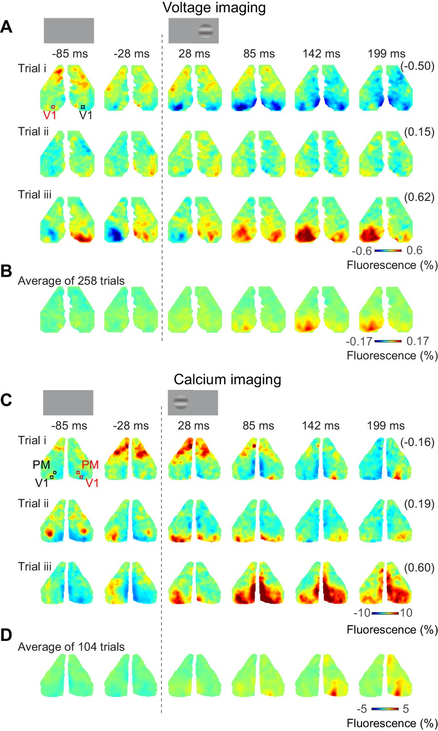
Bilateral ongoing activity continues during unilateral visual responses.
(A) Three example sequences of voltage signal during the period after presentation of 50% contrast to the left monocular visual field in an example mouse expressing VSFP. In each examples, the right-most number in a parenthesis indicates correlation coefficient of the sequence to the average across repeats (B). (B) Average neural activity across repeats. (C, D) Same as (A), (B), for a mouse expressing calcium indicator. The video of activity in these three trials is available at Figure 3—video 1.
Figure 3—video 1
Bilateral ongoing activity continues during unilateral visual responses.
https://doi.org/10.7554/eLife.43533.008
Figure 4
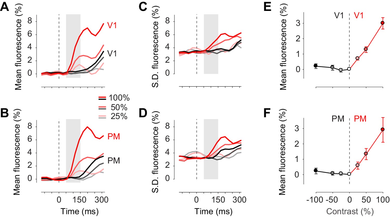
Task stimuli evoke unilateral responses and do not quench bilateral fluctuations.
(A) Mean calcium signal across trials from seven animals in the right stimulated V1 (red) and in the left unstimulated V1 (black). Time period of 50–150 ms after stimulus onset (shaded area) was used for subsequent analysis of visually evoked response. (B) Same as (A) in PM. (C.D) Same as panels (A) and (B) for standard deviation across trials. (E) Average neural activity 50–150 ms after visual stimulation to different contrasts (contrast-response curve) in V1. Activity in the stimulated and unstimulated V1 is shown as red and black lines. Error bars indicate S.E. across seven animals. (F) Same as panel (E) in PM.
Figure 5 with 4 supplements
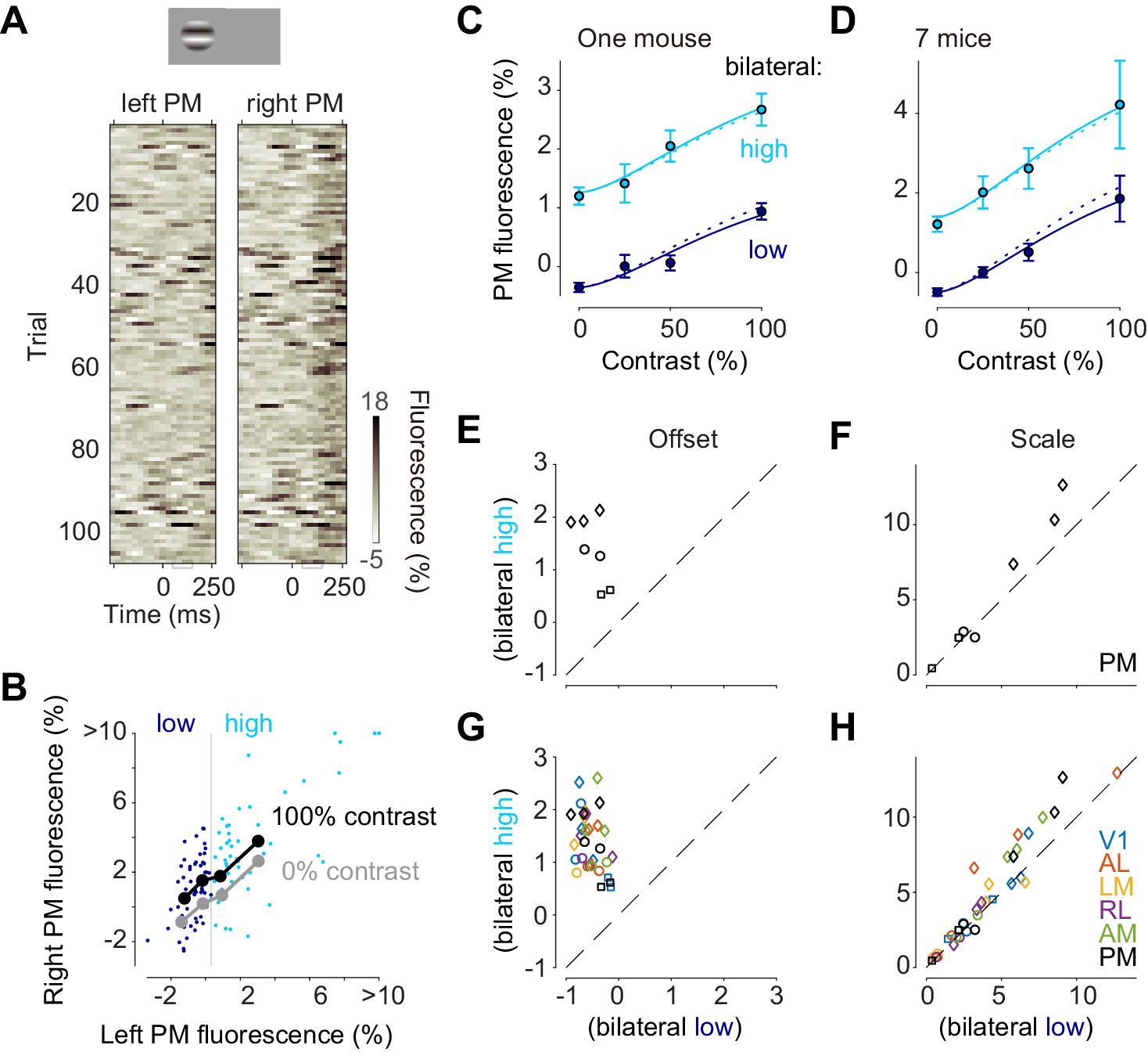
Bilateral ongoing activity and visually evoked responses add linearly.
(A) Single trial traces aligned by the onset of visual stimulation of 100% contrast to the left visual field in the left unstimulated PM and right stimulated PM. The time period (50–150 ms) used for the analysis of visually evoked response is indicated as a gray bracket. (B) Relationship between left PM (abscissa) and right PM (ordinate) 50–150 ms after visual stimulation. Single trial activity to 100% contrast stimulation is shown as cyan and blue dots. Moving average along left PM is shown as thick black (100% contrast) and gray (0% contrast) lines. (C) Contrast responses from trial groups of high (cyan) and low (blue) contralateral ongoing activity in one animal. Data points and error bars indicate median and median absolute deviation across trials from one animal. Curves indicate contrast-response functions where scale parameter is free (solid curve) or fixed (dotted curve) between the high and low ongoing activities. (D) Contrast responses, average of seven animals. Error bars represent S.E. across animals. (E, F) Parameters of contrast-response functions across animals. Offset (E) and scale (F) parameters were estimated individually from trial groups of low (abscissa) and high (ordinate) ongoing activities. Genetic background was Snap25-GCaMP6s (circles), TetO-GCaMP6s;Camk2a-tTA (diamonds) or Vglut1-Cre;Ai95 (squares). (G, H) Same as panels (E) and (F), for all the visual areas.
Figure 5—figure supplement 1
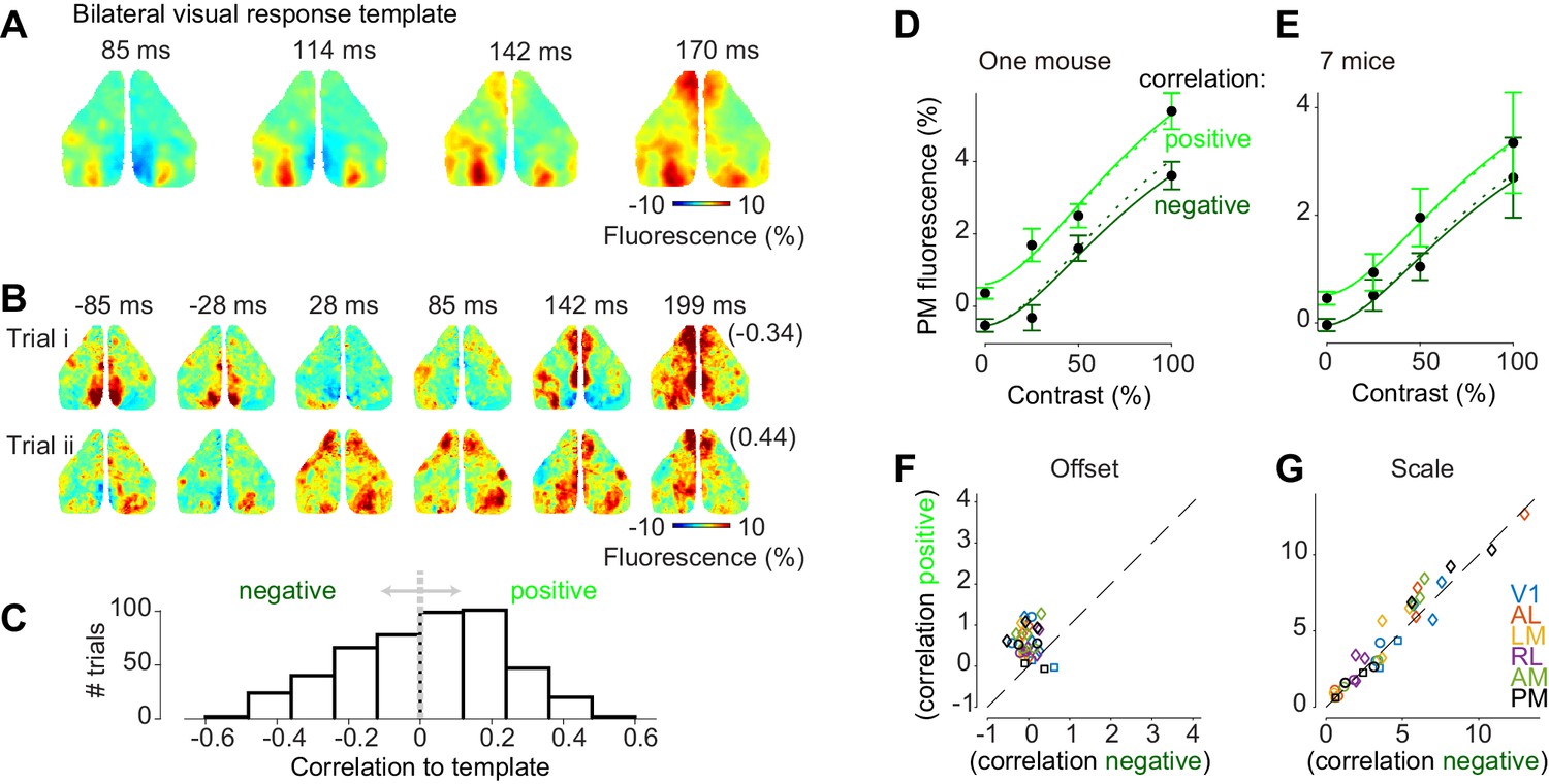
Bilateral ongoing activity and visual responses interact additively regardless of the similarity of their patterns.
(A) Template obtained as average visual response to left and right 100% contrast stimuli obtained from one animal. (B) Example single-trial responses to after presentation of 100% contrast the the right monocular visual field, when ongoing activity at stimulus onset is negatively (top, ρ = −0.34) and positively (bottom, ρ = 0.44) correlated with the template (A). (C) Correlation between single-trial movie and the template, sorted by correlation at stimulus onset. (D) Contrast responses from trial groups of positive (light green) and negative (dark green) visually-evoked motifs at t = 0 in one animal. Data points and error bars indicate median and median absolute deviation across trials from one animal in V1. (E) Contrast responses, average of seven animals. Error bars represent S.E. across animals. (F, G) Parameters of contrast-response functions across animals. Offset (F) and scale (G) parameters were estimated individually from trial groups of negative (abscissa) and positive (ordinate) correlation to visually-evoked motifs.
Figure 5—figure supplement 2
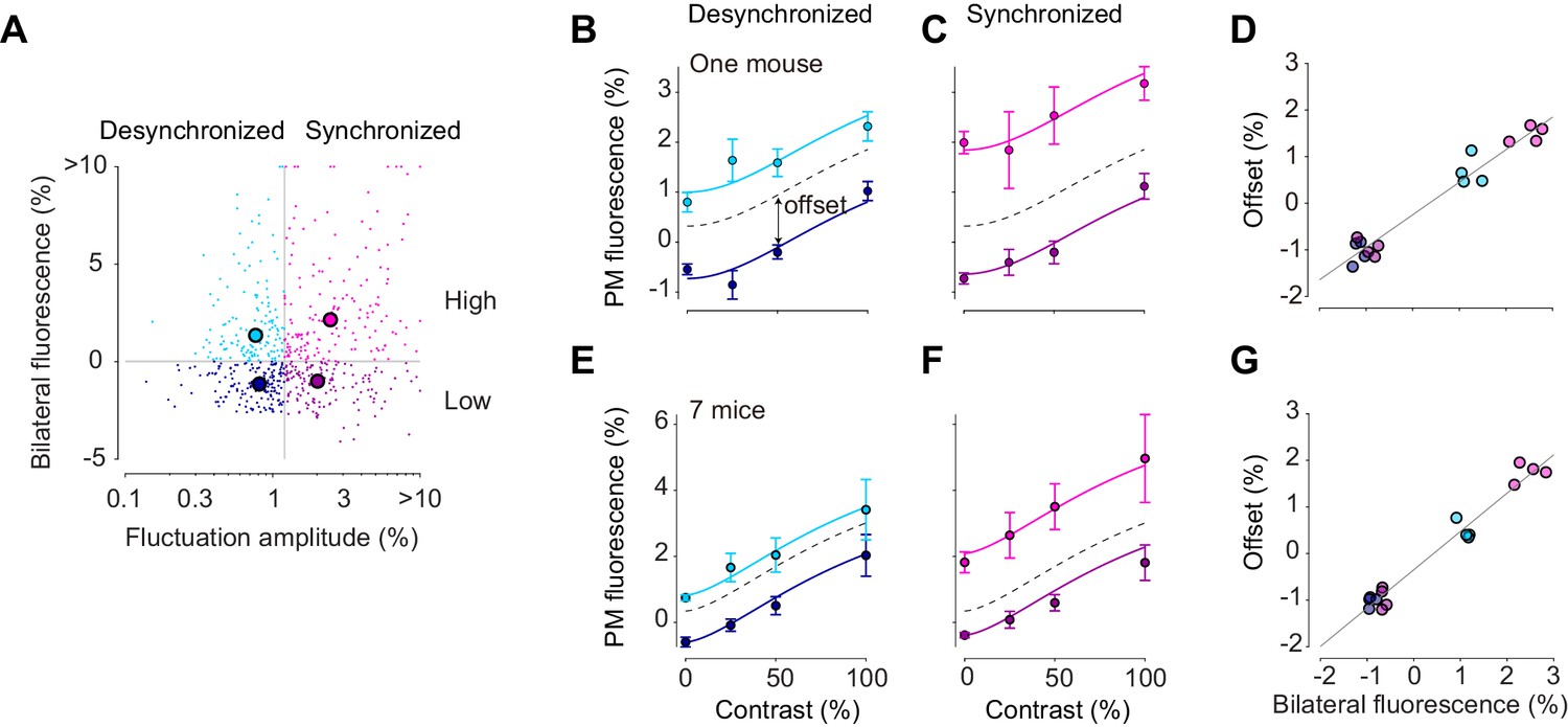
The effects of bilateral ongoing activity were due to fast changes in cortical activation, not to slow changes in cortical state.
(A) Instantaneous amplitude at unstimulated PM (vertical axis) and pre-stimulus fluctuation amplitude between 2–7 Hz at stimulated PM (horizontal axis) of single trials in area PM. Each dot represents single trial drawn from one animal. We then set thresholds to divide trials between ‘Synchronized’ and ‘Desynchronized’ states (vertical line) and between high vs. low instantaneous activity (50–150 ms after stimulus onset, horizontal line). (B) Contrast responses from trials of high (cyan) and low (blue) bilateral ongoing activity in synchronized state in one animal. Black dotted curve indicates grand average across all the trials. Error bars represent median absolute deviation across trials. (C) Contrast responses from trials of high (magenta) and low (purple) bilateral ongoing activity in desynchronized state in one animal. Black dotted curve indicates grand average across all the trials as in panel (B). Error bars represent median absolute deviation across trials. (D) Offset measured as a vertical distance from the grand average curve, against instantaneous amplitude at unstimulated area PM. Symbol colors indicate trial conditions as in panel (A). Each circle represents average across trials in response to different contrasts. (E–G) Same as in panels (B-D) but from averaged data across seven mice.
Figure 5—figure supplement 3
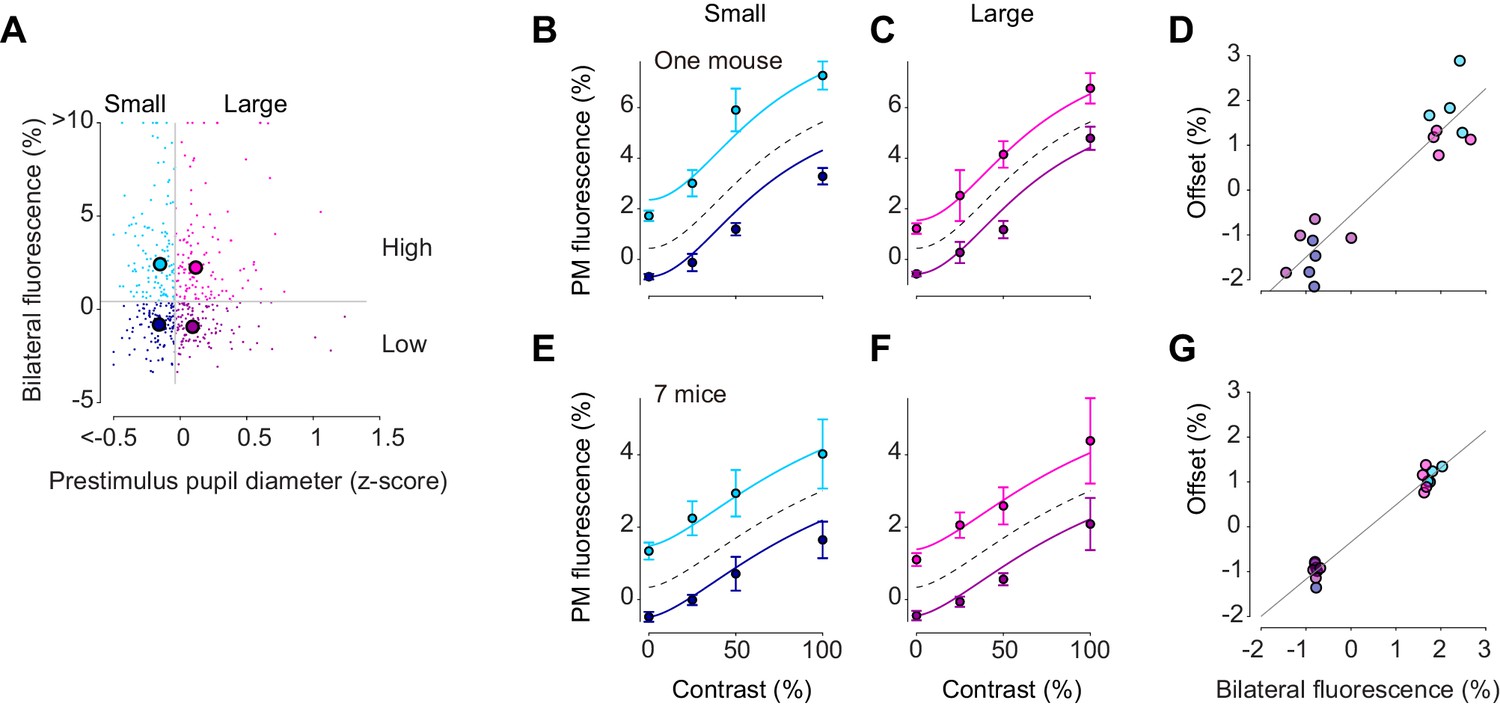
The effects of bilateral ongoing activity were due to fast changes in cortical activation, not to slow changes in pupil diameter.
Same as Figure 5—figure supplement 2, except that trials are divided by prestimulus pupil diameter instead of cortical state.
Figure 5—figure supplement 4
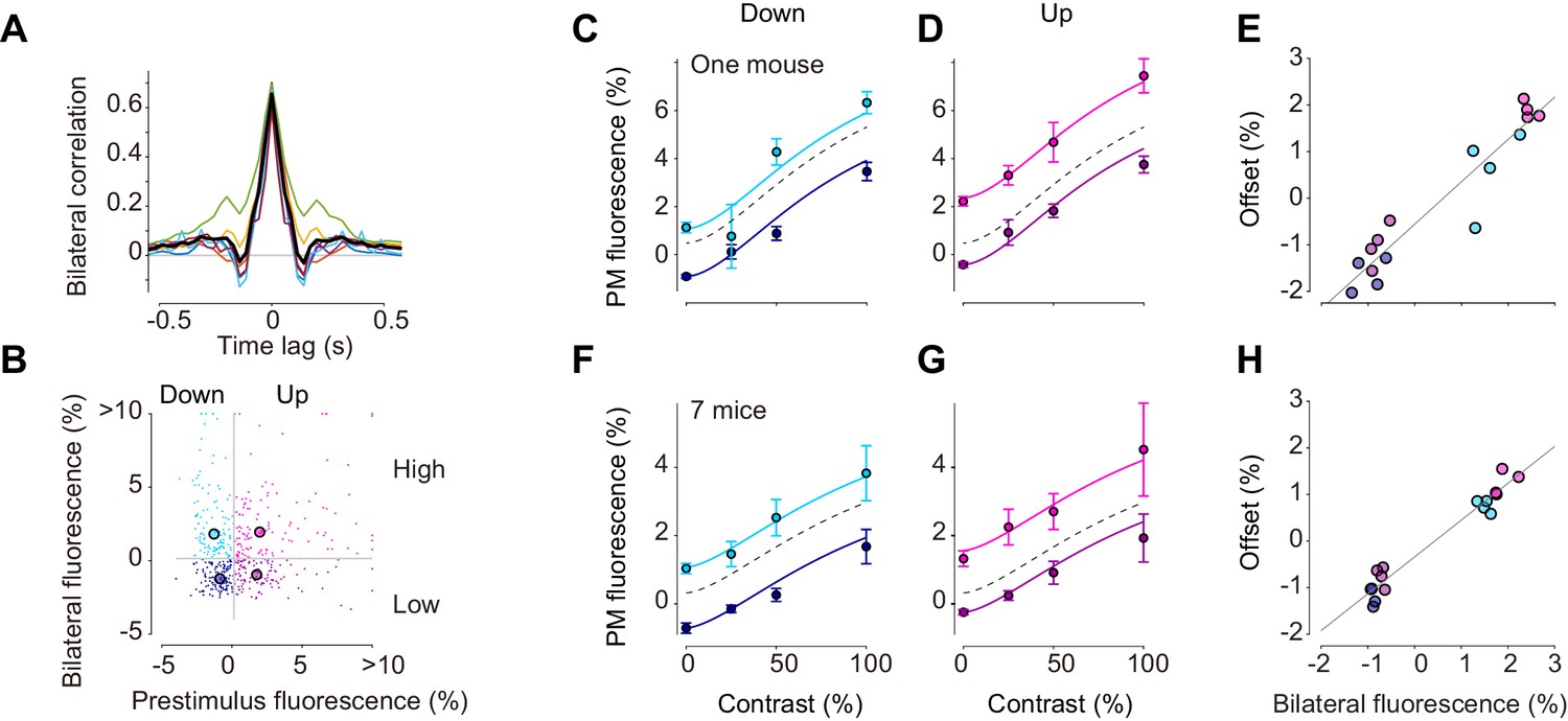
Ongoing activity sampled as prestimulus activity.
(A) Cross-correlation between activity in left and right PM, in individual mice (colored traces) and across all seven mice (black trace). (B) Activities 50–150 ms after visual stimulation of 100% contrast in the stimulated PM (ordinate), against activities 0–100 ms before stimulation in the same ROI (abscissa). Each dot represents single trial activity. (C) Contrast responses from trials of high (cyan) and low (blue) bilateral ongoing activity when prestimulus activity is in Down phase in one animal. Black dotted curve indicates grand average across all the trials. Error bars represent median absolute deviation across trials. (D) Contrast responses from trials of high (magenta) and low (purple) bilateral ongoing when prestimulus activity is in Up phase in one animal. Black dotted curve indicates grand average across all the trials as in panel (B). Error bars represent median absolute deviation across trials. (E) Offset measured as a vertical distance from the grand average curve, against instantaneous amplitude in unstimulated area PM. Symbol colors indicate trial conditions as in panel (B) Each circle represents average across trials in response to different contrasts. (F–H) Same as in panels (B-D) but from averaged data across seven mice.
Figure 6 with 1 supplement

Bilateral ongoing activity does not affect perceptual reports.
(A) Probability of turning the wheel to the correct direction as a function of stimulus contrast in one animal. The probability is computed separately in trial groups of low (blue) and high (cyan) ongoing activity measured in area PM. Error bars indicate 95% binomial confidence intervals. Curves indicate psychometric functions obtained by fitting a probabilistic observer model (Burgess et al., 2017) separately to the two sets of responses. (B) Same as (A), for probability of no-go. (C, D) Same as (A), (B), averaged across mice. Error bars represent S.E. across seven mice. (E) Offset parameter of the perceptual contrast sensitivity function inferred by the model, measured when bilateral activity in PM was low (abscissa) vs. high (ordinate). Symbols indicate parameters from individual animals. Genetic background was Snap25-GCaMP6s (circles), TetO-GCaMP6s;Camk2a-tTA (diamonds) or Vglut1-Cre;Ai95 (squares). (F Same as E), for all visual areas. (G, H) Same as (E), (F), for the scale parameter of the perceptual contrast sensitivity function.
Figure 6—figure supplement 1
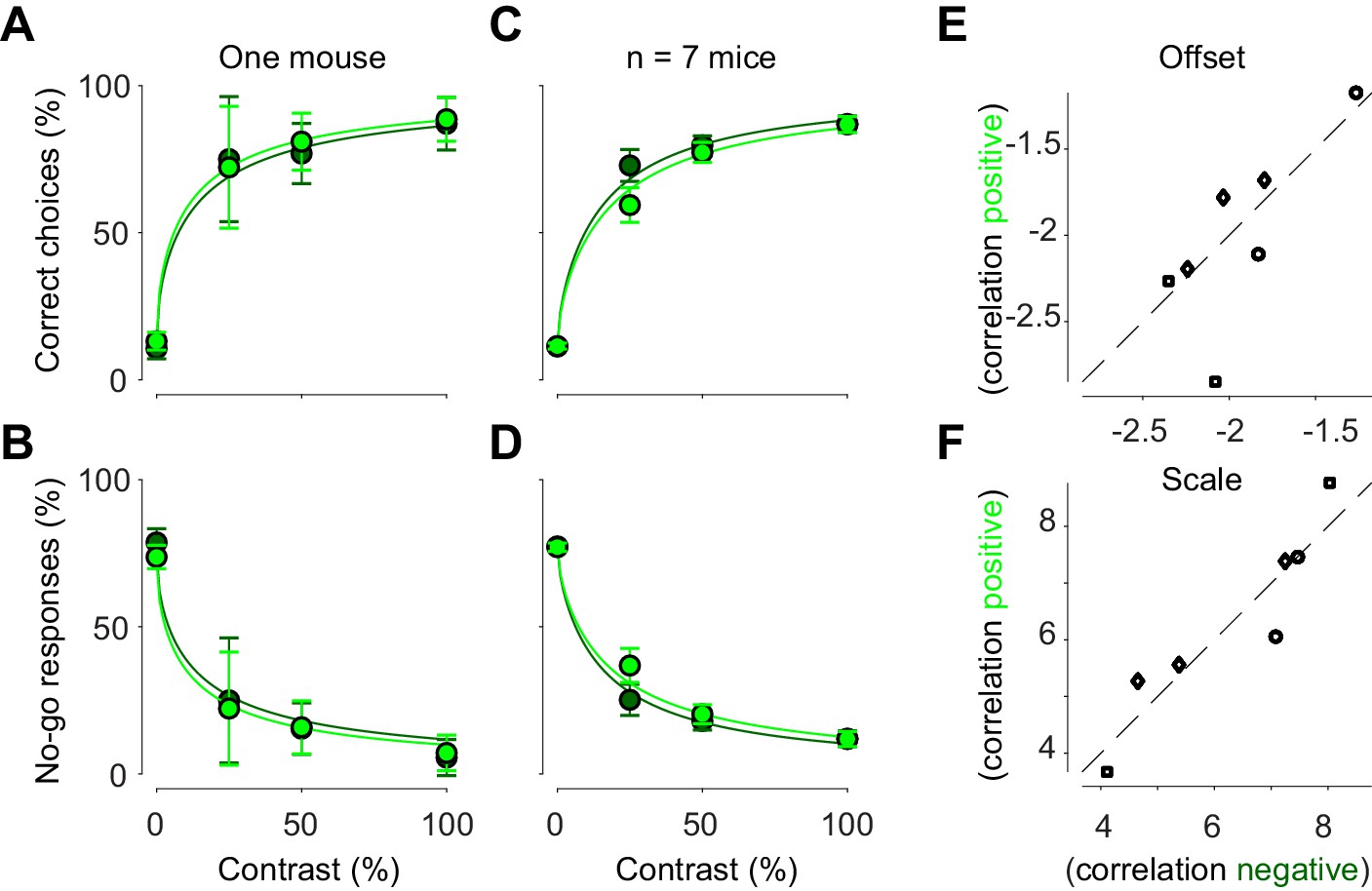
Bilateral ongoing motif does not affect perceptual reports.
(A) Probability of turning the wheel to the correct direction as a function of stimulus contrast in one animal. The probability is computed separately in trial groups of negative (dark green) and positive (light green) correlation to visually evoked motifs. Error bars indicate 95% binomial confidence intervals. Curves indicate psychometric functions obtained by fitting a probabilistic observer model (Burgess et al., 2017) separately to the two sets of responses. (B) Same as (A), for probability of no-go. (C, D) Same as (A) and (B), averaged across mice. Error bars represent S.E. across seven mice. (E) Offset parameter of the perceptual contrast sensitivity function inferred by the model, measured when correlation between ongoing activity and visually evoked motif was negative (abscissa) vs. positive (ordinate). Symbols indicate parameters from individual animals. Genetic background was Snap25-GCaMP6s (circles), TetO-GCaMP6s;Camk2a-tTA (diamonds) or Vglut1-Cre;Ai95 (squares). (F) Same as (E), for the scale parameter.
Figure 7 with 1 supplement

Additive model accounts most trial-by-trial variations in visual responses.
(A) Schematic representation of the additive model (Equation 1). (B) Single-trial PM traces predicted by the additive model. (B1) bilateral activity, estimated from left PM. (B2) visually evoked response of the right PM, estimated as average across trials of right PM. (B3) predicted activity of the right PM by the additive model. (B4) observed activity of the right PM. (B5) difference between predicted and observed activity in right PM. (C) Variance of activity in PM explained by the additive model, as a function of distance from location of PM to location of ROI used as a regressor. Circles represent average across animals. Gray curve indicates a result of exponential fit. (D) Variance explained by the visually evoked and bilateral activities (additive model, red), and by the visually evoked activity alone (black). Circles and error bars indicate average and S.E. across animals. Dots represent different animals. (E) As in (C), for voltage signals (n = 2 mice). Circles represent average across animals. (F aAs in D) for voltage signals (circles, n = 2 mice).
Figure 7—figure supplement 1
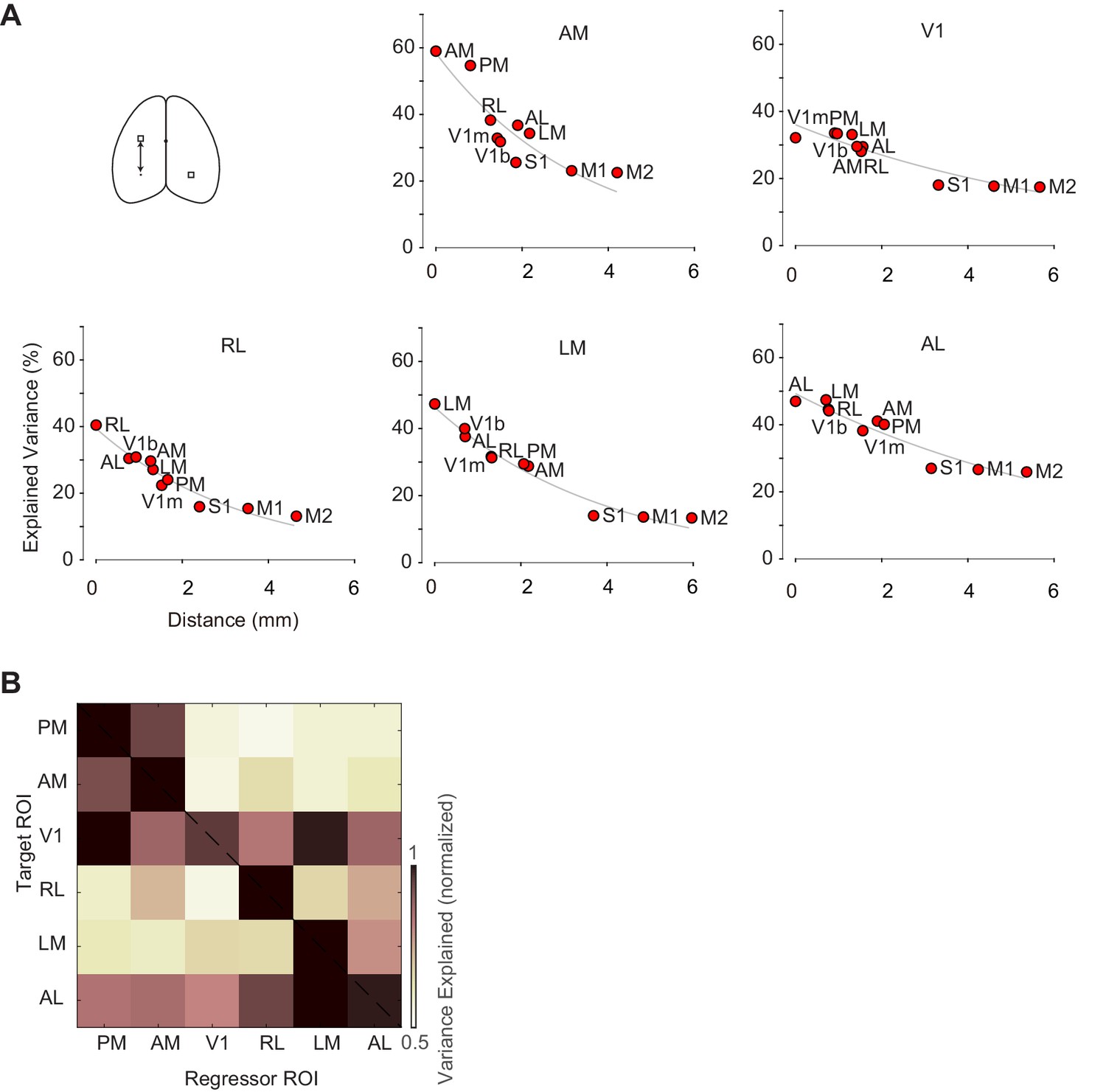
Variance explained by the additive model in different visual areas.
(A) Variance of activity in each visual area explained by the additive model, as a function of distance from location of the corresponding area in the other hemisphere. Gray curves indicate results of exponential fit. (B) Variance explained by the additive model using different ROIs as regressors (abscissa). Variance was normalized in each target ROI across regressor ROIs, by dividing maximum explained variance.
Author response image 1
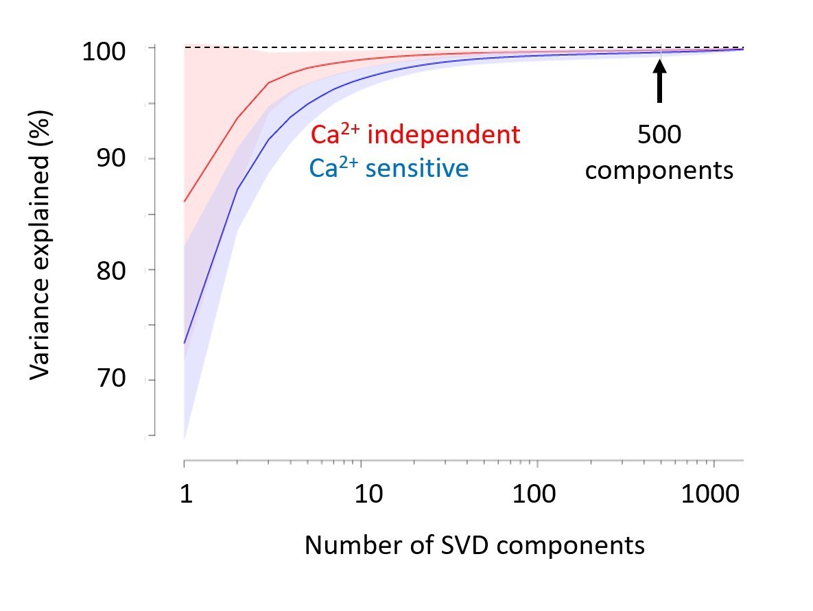
Singular Value Decomposition efficiently compresses calcium-imaging data.
A few tens of components are sufficient to capture close to 100% of the variance, both in the calcium-sensitive channel (blue) and in the calcium-independent channel (red). In the paper, we use 500 components (arrow). Shaded area represents s.d. across imaging sessions. Similar results were obtained with Voltage-Sensitive Fluorescent Protein imaging.
Author response image 2
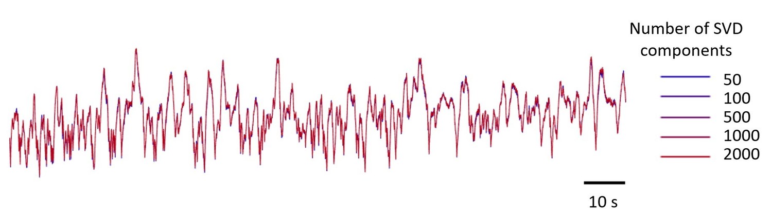
Example GCaMP traces in V1, using 5 numbers of SVD components, from 50 to 2,000 components.
The resulting five traces look identical. The number of components used in the paper is 500.
Author response image 3
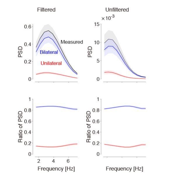
Bandpass filtering the signals does not affect the estimate of bilateral activity.
Left: Results obtained after taking the derivative and lowpass filtering (as used in our paper). Right: Results obtained without any filtering. By definition, filtering affects the power spectral density (top). However, the relative strength of bilateral activity (relative to total) remains the same, independent of frequency (bottom). We now show the bottom left panel in Figure 1.
Additional files
-
Transparent reporting form
- https://doi.org/10.7554/eLife.43533.019
Download links
A two-part list of links to download the article, or parts of the article, in various formats.
Downloads (link to download the article as PDF)
Open citations (links to open the citations from this article in various online reference manager services)
Cite this article (links to download the citations from this article in formats compatible with various reference manager tools)
The impact of bilateral ongoing activity on evoked responses in mouse cortex
eLife 8:e43533.
https://doi.org/10.7554/eLife.43533


