Automated cryo-EM structure refinement using correlation-driven molecular dynamics
- Max Planck Institute for Biophysical Chemistry, Germany
Figures
Figure 1
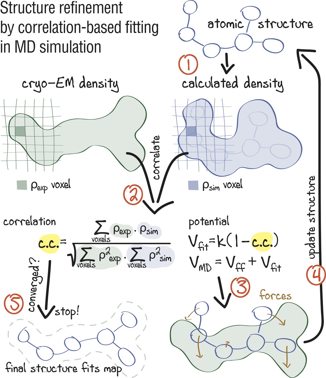
Approach: using correlation-based refinement in MD simulation to steer the atomic positions of a macromolecule such that they optimally fit a cryo-EM map.
The molecule is subjected to a global biasing potential in addition to the MD force field . The forces resulting from act on every atom to enhance the real-space correlation coefficient between the cryo-EM density (green) and the density calculated from the current atomic positions (blue). The first step (1) is to generate a simulated density by convoluting the atomic positions with a three-dimensional Gaussian function of width (Orzechowski and Tama, 2008). The two maps are correlated (2), and the biasing forces are calculated. These forces are then added to the standard MD force field (3), and new atomic positions are evaluated (4). Steps (1–4) are repeated, yielding a structure that correlates better with the cryo-EM map than the starting structure.
Figure 2 with 1 supplement

Schematic representation of the proposed continuous refinement protocol: (1) a low temperature optimization phase, where is monotonously increased by increasing the force constant (columns a–d), followed by (2) simulated annealing (columns e, f).
The local effect of the protocol is exemplified in the upper row for a one-dimensional single-atom case. Simulated densities shown in the middle row were generated using the atomic structure of a tubulin dimer (PDB ID: 3JAT; Zhang and Nogales, 2015).
Figure 2—figure supplement 1
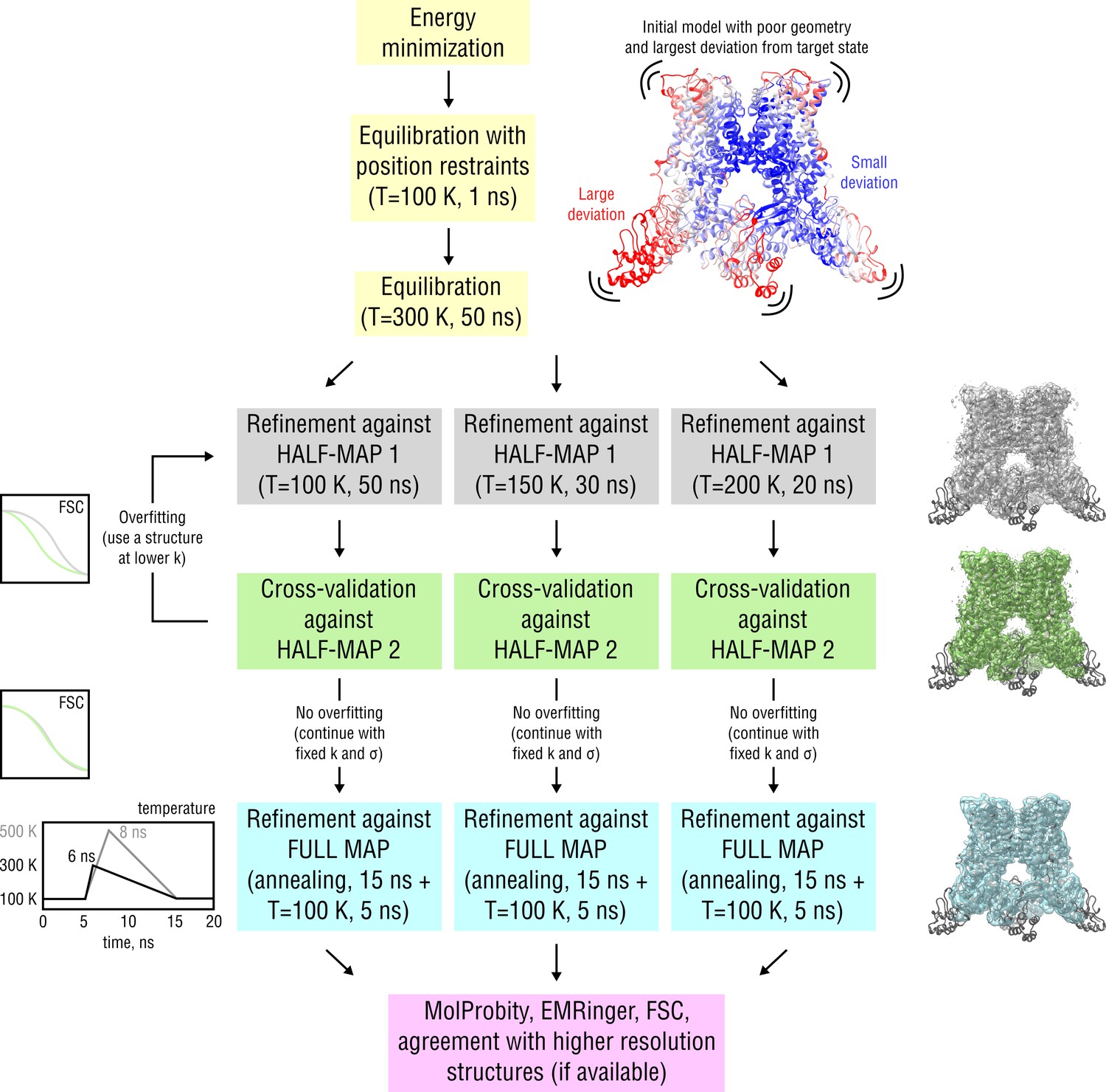
Detailed scheme of the proposed continuous refinement protocol subdivided in five stages.
In stage 1 (yellow), the starting structure is subjected to initial equilibration in explicit solvent. Equilibration at = 300 K for 50 ns is needed to drive the starting structure further away from the target state, posing an additional refinement challenge. In real applications, a short equilibration run at = 100 K for 5–10 ns should be sufficient. Stages 2 and 3 (gray and green) include the refinement against one of the half-maps (training map) followed by cross-validation by means of Fourier Shell Correlation (FSC) against the other half-map (validation map). In case no overfitting of the training map is observed, the final structure from the half-map refinement is passed to stage 4 (cyan), where it is refined against the full map to account for high-resolution features not present in both half-maps. Finally, in stage 5 (purple), the average structure from the last 5 ns of the full map refinement is subjected to geometry and goodness-of-fit assessment. Note that the procedure is automated such that stages 1–4 can be run without human intervention. Pausing the refinement to inspect intermediate results or introduce changes to the protocol should be possible at any stage. See Materials and methods for more details.
Figure 3 with 2 supplements
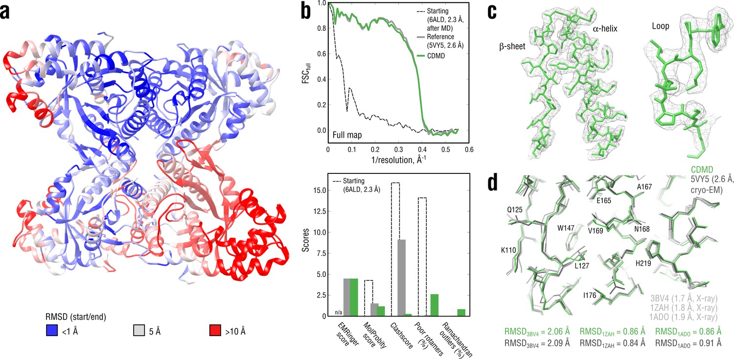
Refining a distant starting model into a high-resolution map: rabbit muscle aldolase at 2.6 Å.
(a) RMSD (Cα atoms) between the starting and the reference model (5VY5) showing the extent of rearrangements during refinement. (b) Reciprocal-space agreement of the starting (black dashed), the reference (gray) and our refined model (green) with the full map (top) and stereochemical quality for the three models assessed by EMRinger and MolProbity (bottom). (c) Representative secondary structure elements showing local agreement of our model with the full map. (d) Representative region of the protein interior (chain A) showing the closeness of our model and the reference to higher resolution control X-ray structures in terms of RMSD. Some residues are explicitly labeled.
Figure 3—figure supplement 1
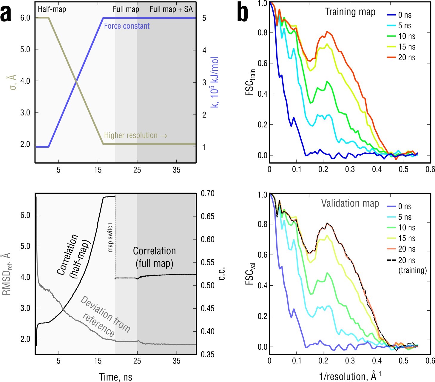
Extension of Figure 3 showing the time evolution of various characteristics during refinement.
(a) The simulated map resolution and force constant were linearly ramped from 0.6 nm and 0.5 × 10⁵kJ mol-1 to the target values of 0.2 nm and 5 × 10⁵ kJ mol-1, respectively. At the bottom, the time evolution of with the training and the full map and RMSD to the reference structure are shown. (b) FSCtrain and FSCval sampled every five ns. Cross-validation showed no signs of overfitting (black dashed lines).
Figure 3—figure supplement 2

Extension of Figure 3 showing the comparison of the radii of convergence across different refinement methods for the aldolase system and using the same distant starting structure.
RMSD to the reference structure for all methods used is shown in the upper left plot. Overlays between the reference (gray) and the refined structures are depicted as ribbons (colors as in the RMSD plot).
Figure 4 with 1 supplement
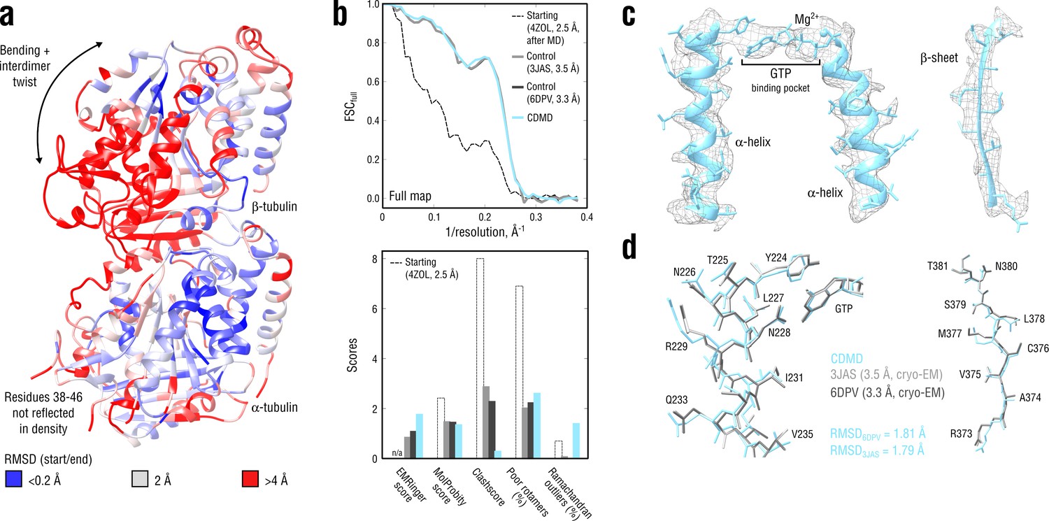
Refinement of a curved tubulin dimer into a map of the straight, microtubule-like state.
(a) RMSD (Cα atoms) between the starting and the control model (6DPV) showing the extent of rearrangements between the solution (curved) and the microtubule-like (straight) tubulin conformation. The -subunits of both models were aligned for the RMSD calculation. (b) Reciprocal-space agreement of the starting (black dashed), the control (gray and dark gray) and our model (cyan) with the full map (top) and stereochemical quality for the four models assessed by EMRinger and MolProbity (bottom). (c) Representative secondary structure elements showing local agreement of our model with the full map. (d) Same as in c but showing the closeness of our model to higher resolution control structures in terms of RMSD. Some residues are explicitly labeled.
Figure 4—figure supplement 1
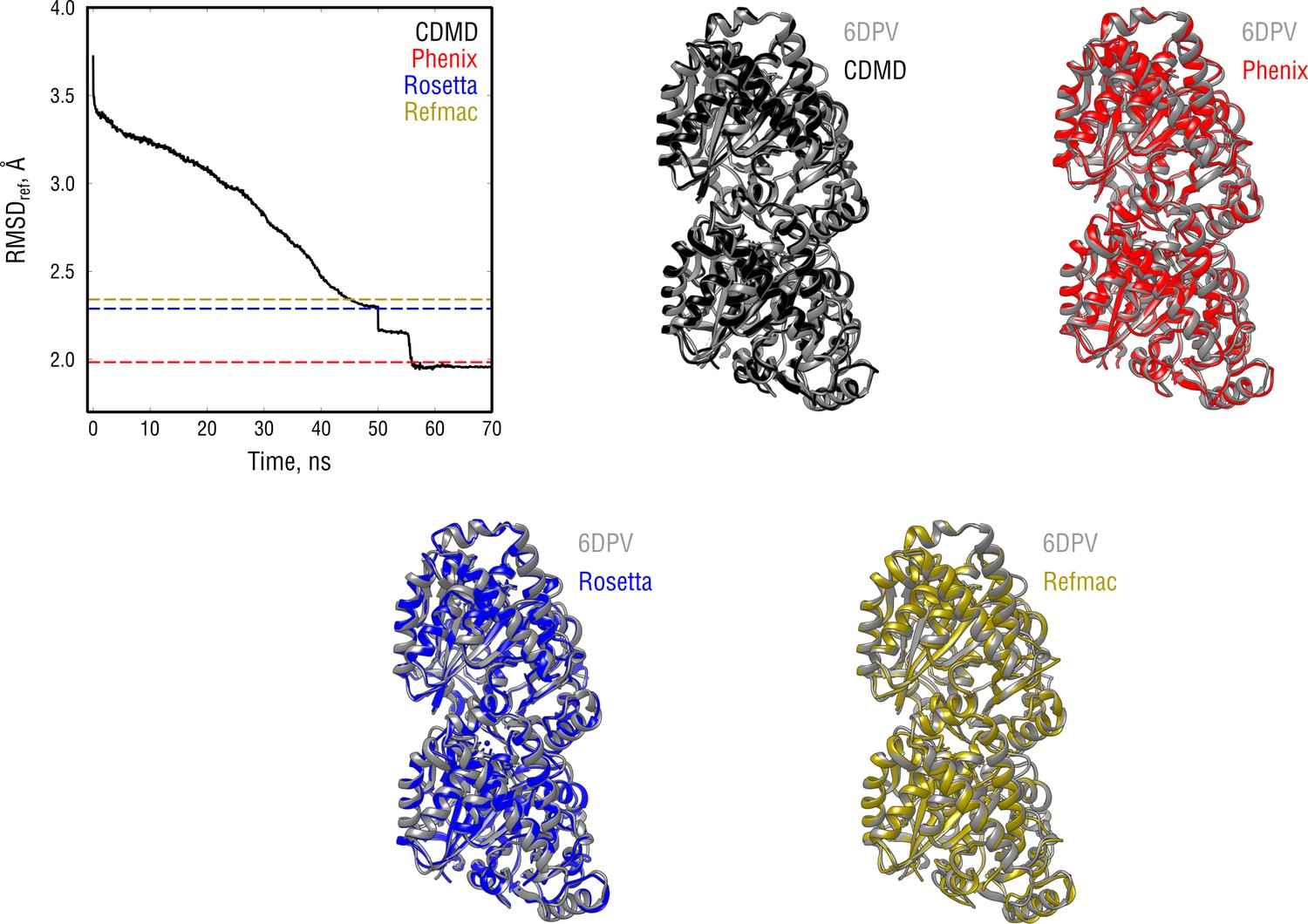
Extension of Figure 4 showing the comparison of the radii of convergence across different refinement methods for the tubulin system and using the same distant starting structure.
RMSD to the reference structure for all methods used is shown in the upper left plot. Overlays between the control (6DPV, gray) and the refined structures are depicted as ribbons (colors as in the RMSD plot).
Figure 5 with 2 supplements

Refinement of a poor structure of TRPV1 in a distant conformation into a map with highly heterogeneous local resolution.
(a) RMSD (Cα atoms) between the starting and the reference model (3J5P) showing the extent of rearrangements the TRPV1 structure undergoes during refinement. (b) Reciprocal-space agreement of the starting (black dashed), the reference (gray) and our model (purple) with the full map (top) and stereochemical quality of the models assessed by EMRinger and MolProbity (bottom). Note that the starting model was derived from the deposited structure by subjecting the latter to MD at = 300 K. (c) Representative secondary structure elements showing local agreement between of our model with the full map.
Figure 5—figure supplement 1
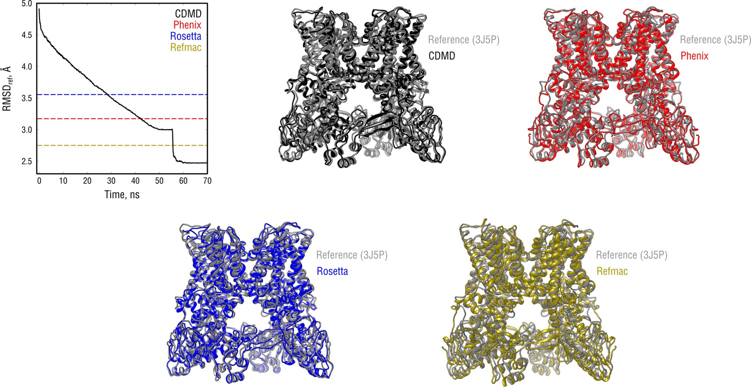
Extension of Figure 5 showing the comparison of the radii of convergence across different refinement methods for the TRPV1 system and using the same distant starting structure.
RMSD to the reference structure for all methods used is shown in the upper left plot. Overlays between the reference (3J5P, gray) and the refined structures are depicted as ribbons (colors as in the RMSD plot).
Figure 5—figure supplement 2
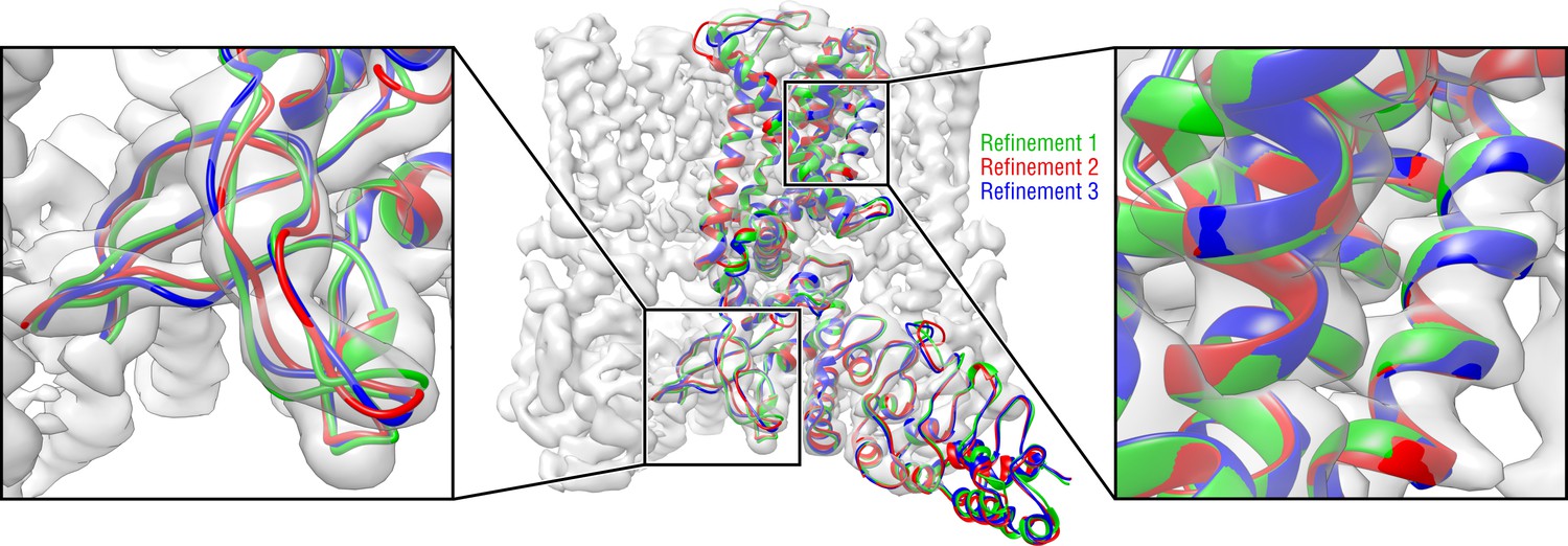
Convergence of the TRPV1 refinement both in the higher resolution TM region and in the lower resolution ARD region assessed by means of three independent refinement runs using different but similarly distant starting structures.
Only one TRPV1 monomer and no side chains are shown for clarity.
Figure 6
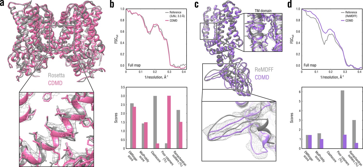
Comparison of our TRPV1 model with those previously refined using Rosetta (a, b) and ReMDFF (c, d).
Overlays of our model (pink and violet ribbon) with the Rosetta (left, gray ribbon) and ReMDFF (right, gray ribbon) models are shown in (a) and (c), respectively. Reciprocal-space agreement with the full map (top) and stereochemical quality for the four models assessed by EMRinger and MolProbity (bottom) are shown in (b) for the Rosetta model and in (d) for the ReMDFF model.
Figure 7 with 1 supplement
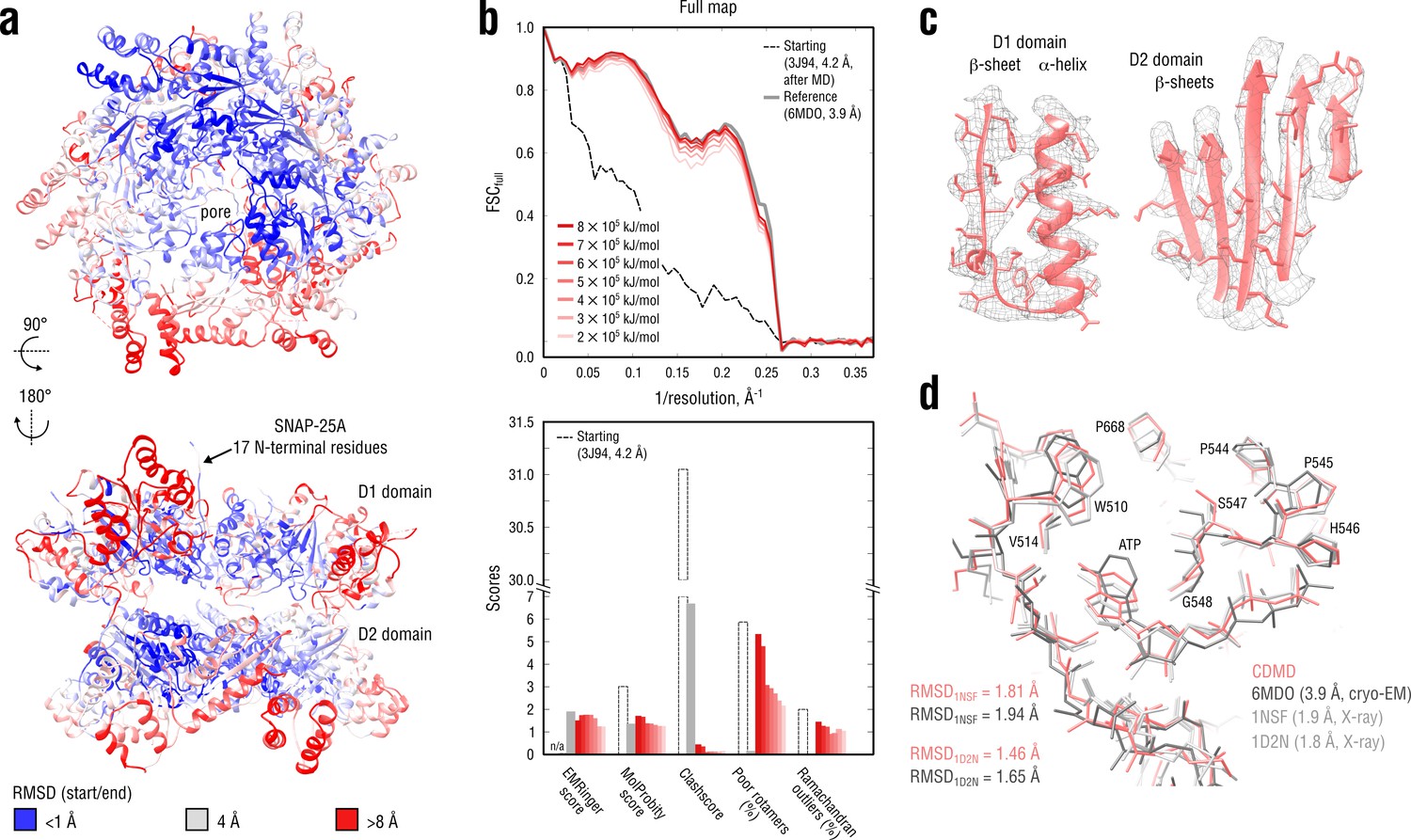
Refinement of a substrate-free NSF complex in a distant conformation into a medium-resolution map at 3.9 Å.
(a) RMSD (Cα atoms) between the starting and the reference model (6MDO) showing the extent of rearrangements the NSF structure undergoes during refinement. (b) Reciprocal-space agreement with the full map for the starting (black dashed), the reference (gray) and the set of final models (red gradient) refined using a wide range of target force constants (top) and stereochemical quality assessed by EMRinger and MolProbity (bottom). (c) Representative secondary structure elements showing local agreement of the model refined at = 5 105 kJ mol-1 with the map. (d) ATP binding pocket of the D2 domain (chain A) showing the closeness of our model and the reference to higher-resolution control X-ray structures in terms of RMSD. Some residues are explicitly labeled.
Figure 7—figure supplement 1
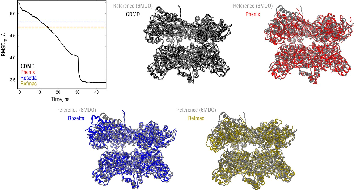
Extension of Figure 7 showing the comparison of the radii of convergence across different refinement methods for the NSF system and using the same distant starting structure.
RMSD to the reference structure for all methods used is shown in the upper left plot. Overlays between the reference (6MDO, gray) and the refined structures are depicted as ribbons (colors as in the RMSD plot).
Figure 8 with 2 supplements
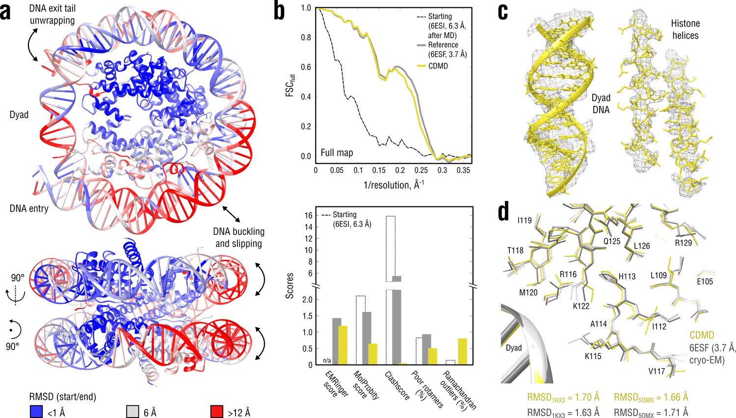
Refinement of a distant nucleosome structure into a medium-resolution map of the canonical nucleosome state.
(a) RMSD (DNA and protein backbone) between the starting and the reference model (6ESF) showing the extent of rearrangements during the refinement. (b) Reciprocal-space agreement of the starting (black dashed), the reference (gray) and our model (yellow) with the full map (top) and stereochemical quality assessed by EMRinger and MolProbity (bottom). (c) Representative secondary structure elements showing local agreement of our model with the full map. (d) Representative region next to the dyad DNA showing the closeness of our model to higher-resolution control structures in terms of RMSD (only protein non-hydrogen atoms). Some residues are explicitly labeled.
Figure 8—figure supplement 1
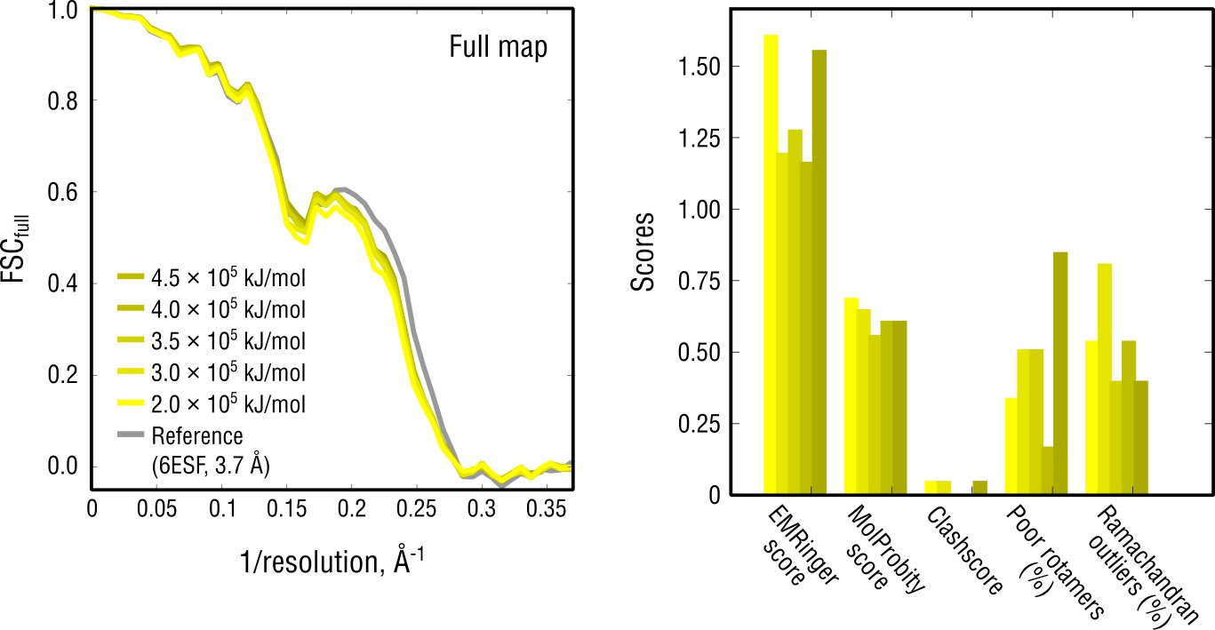
Extension of Figure 8b showing the reciprocal-space agreement and stereochemical quality for nucleosome models independently refined using force constants ranging from 2 to 4.5 105 kJ mol-1.
The structure shown in Figure 8 was refined using = 3 105 kJ mol-1.
Figure 8—figure supplement 2
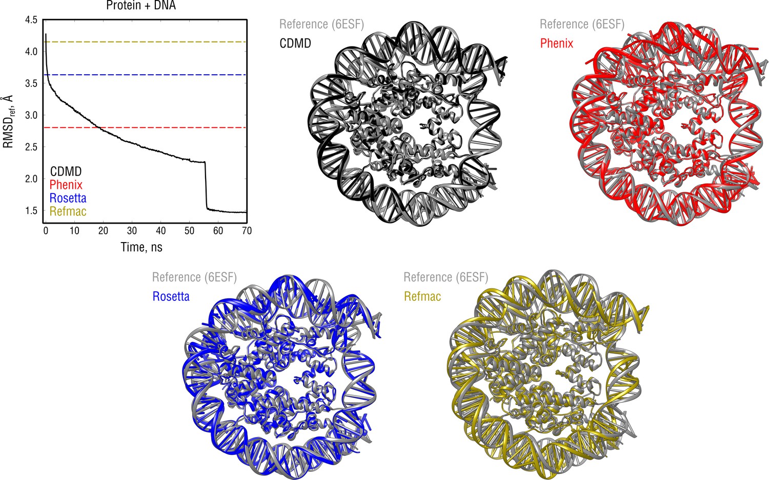
Extension of Figure 8 showing the comparison of the radii of convergence across different refinement methods for the nucleosome system and using the same distant starting structure.
RMSD to the reference structure for all methods used is shown in the upper left plot. Overlays between the reference (6ESF, gray) and the refined structures are depicted as ribbons (colors as in the RMSD plot).
Figure 9 with 2 supplements
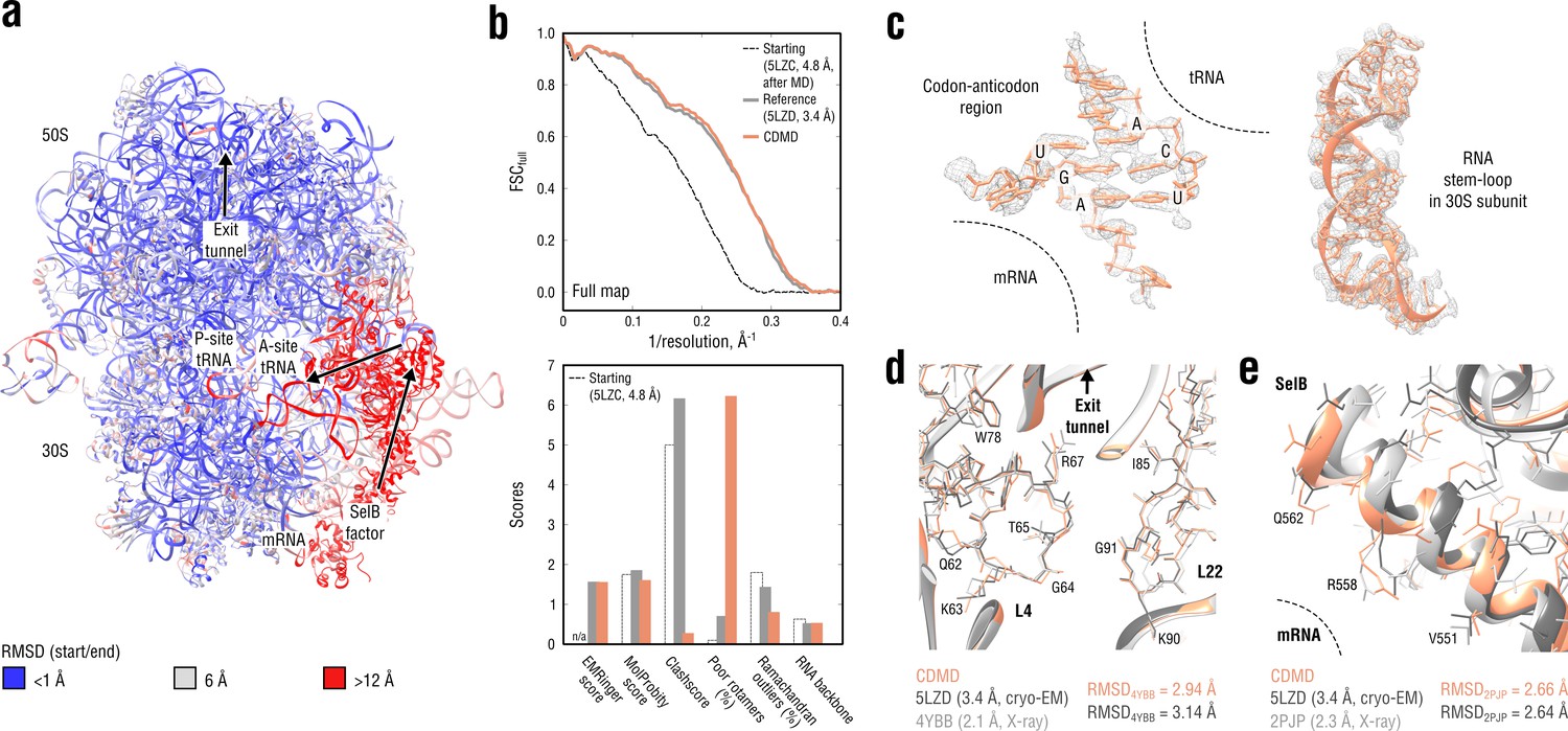
Refinement of a ribosome complex in the CR state into a 3.4 Å map of the GA state.
(a) RMSD (RNA and protein backbone) between the starting (CR) and the final (GA) model showing the extent of rearrangements during the refinement. (b) Reciprocal-space agreement of the starting (black dashed), the reference (gray) and our model (orange) with the full map (top) and stereochemical quality for the three models assessed by EMRinger and MolProbity (bottom). (c) Representative regions showing local agreement between our model and the map (the codon-anticodon region and a RNA stem-loop in the 30S subunit). (d, e) Representative regions in the ribosomal exit tunnel (constriction site formed by L4 and L22 protein chains is shown) and in the SelB-mRNA contact interface, both demonstrating the closeness of our model to higher resolution control structures in terms of RMSD. Some protein residues are explicitly labeled.
Figure 9—figure supplement 1
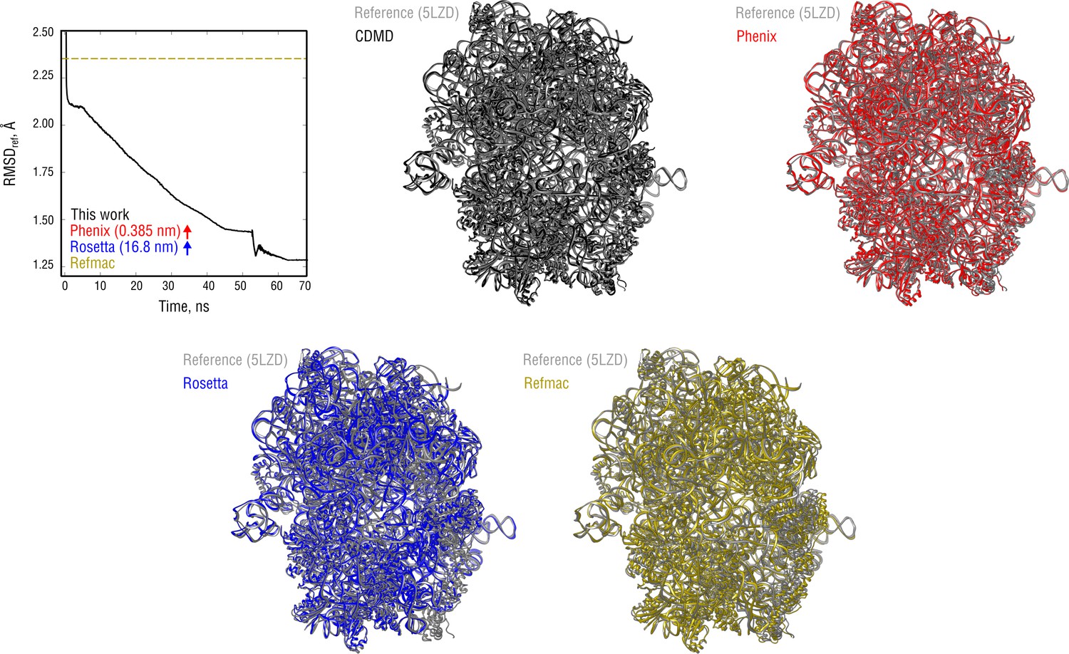
Extension of Figure 9 showing the comparison of the radii of convergence across different refinement methods for the ribosome system and using the same distant starting structure.
RMSD to the reference structure for all methods used is shown in the upper left plot. Overlays between the reference (5LZD, gray) and the refined structures are depicted as ribbons (colors as in the RMSD plot).
Figure 9—video 1
Refinement trajectory for the 70S ribosome.
https://doi.org/10.7554/eLife.43542.021
Figure 10 with 3 supplements
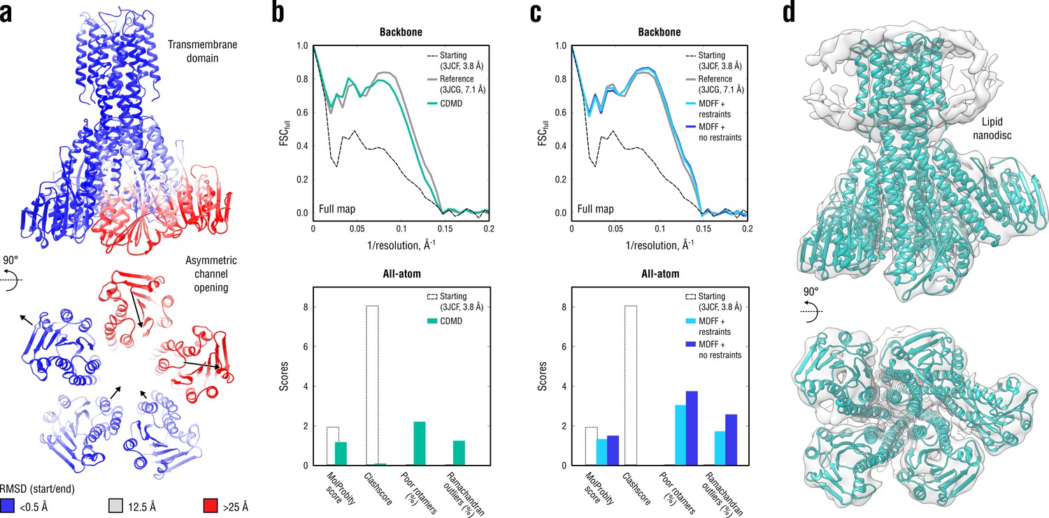
Refinement of a CorA magnesium transporter in the symmetric closed state into a low-resolution 7.1 Å map of the asymmetric open state.
(a) RMSD (Cα atoms) between the starting (closed) and the reference (open) model showing the extent of rearrangements in the cytosolic part of the channel during refinement. (b) Reciprocal-space agreement of the starting (black dashed), the reference (gray) and our model refined with 1.0 105 kJ mol-1 (sea green) with the full map (top) and stereochemical quality for the three models assessed by EMRinger and MolProbity (bottom). The FSC curves were calculated using the backbone atoms only, whereas the full-atom models were used for geometry analysis. No EMRinger scores were calculated. (c) Same as in (b) but for the two MDFF models refined with (blue) and without (dark blue) secondary structure, chirality and cis peptide bond restraints. (d) Overlay of our full-atom model (see green) with full map.
Figure 10—figure supplement 1
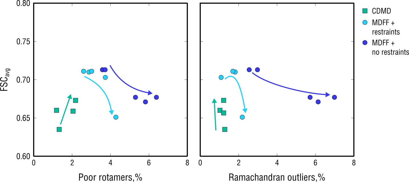
Extension of Figure 10 showing map-model agreement vs. rotamer or Ramachandran outliers for all CDMD and MDFF refinements.
Average FSC values (FSCavg) were calculated as described in Materials and methods. Each dot represents the result of a single independent refinement. MDFF force constants ranged from 0.05 to 0.5 (see Materials and methods for the MDFF protocol). Arrows indicate the trend in FSCavg, rotamer and Ramachandran outliers as the force constant increases.
Figure 10—figure supplement 2
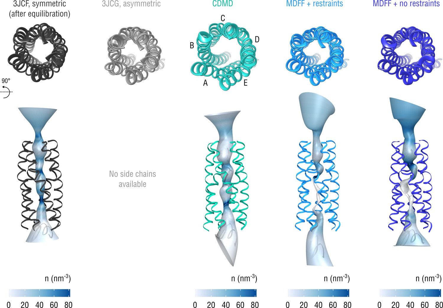
Extension of Figure 10 showing the structure of the gating pore.
The pore transmembrane helices (residues 281–312) are shown for clarity.
Figure 10—figure supplement 3
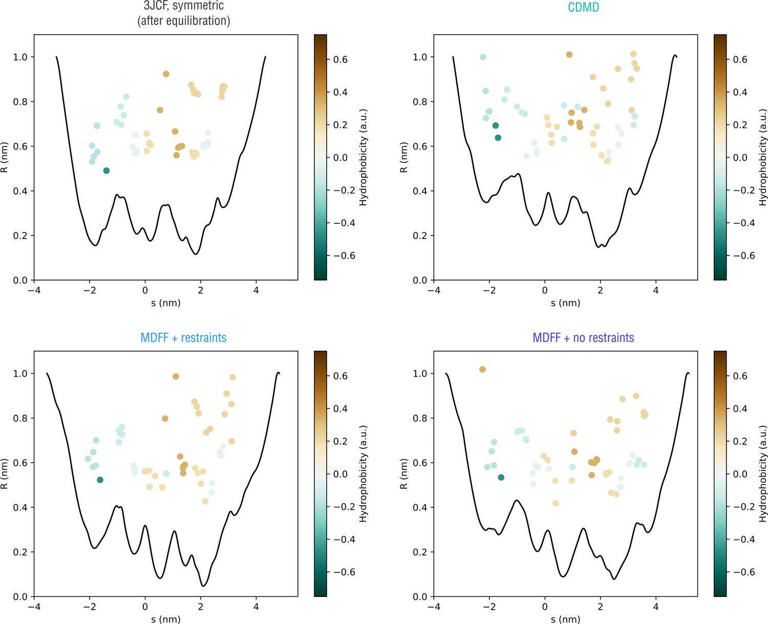
Extension of Figure 10 showing how the pore radius changes along the nonlinear gating pathway showin in Figure 10—figure supplement 2 (bottom).
Residues facing the gating pathway are shown as dots color-coded by their relative hydrophobicities.
Figure 11
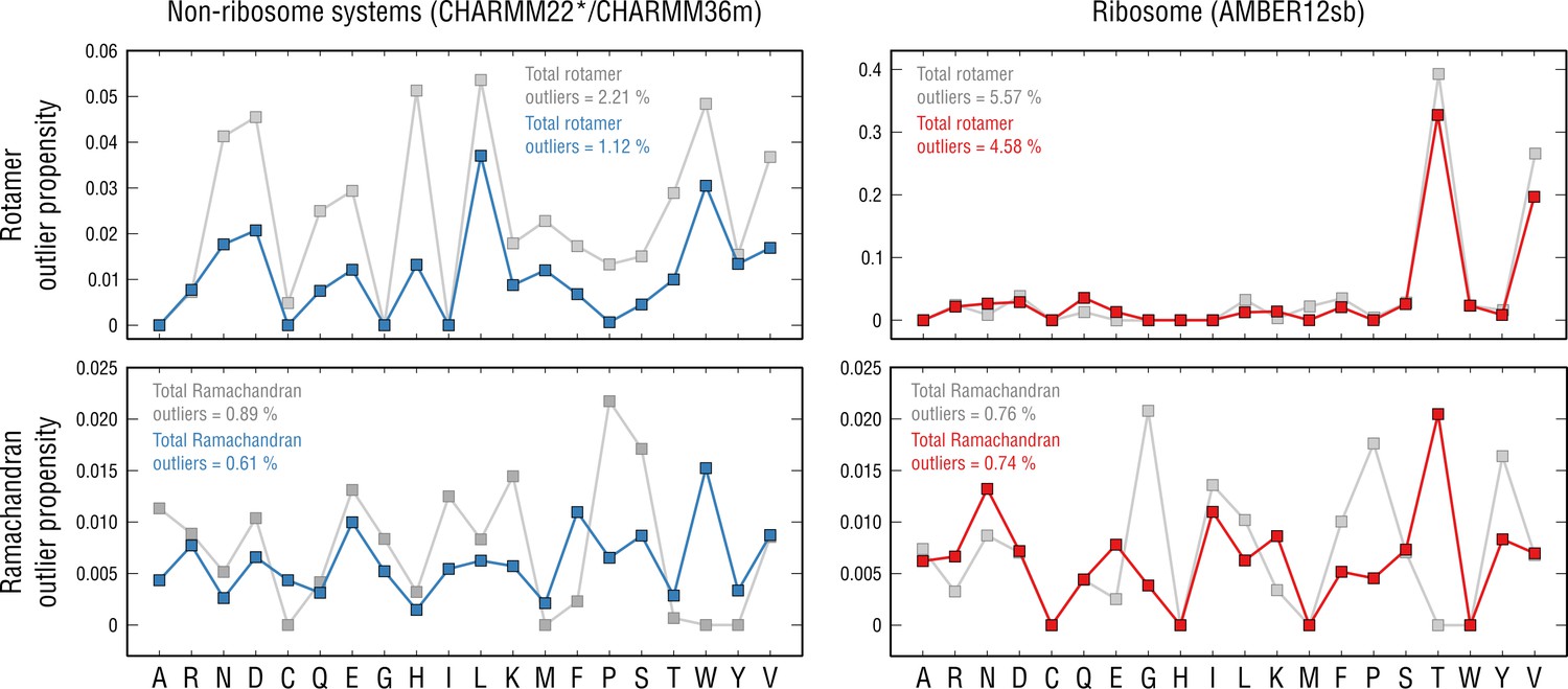
Per-residue outlier analysis.
Per-residue rotamer and Ramachandran outlier propensities calculated from the non-ribosome structures (left panels; CHARMM22*/CHARMM36m force fields were used (Piana et al., 2011; Huang et al., 2017) and the ribosome structure (right panels; AMBER12sb was used; Lindorff-Larsen et al., 2010) after pre-equilibration with the force field (gray dots) and after the actual refinement with our approach (blue and red dots, respectively).
Tables
Table 1
Refinement statistics for the aldolase system.
https://doi.org/10.7554/eLife.43542.029| CDMD | Phenix | Rosetta | Refmac | |
|---|---|---|---|---|
| FSCavg (full map) | 0.774 | 0.704 | 0.790 | 0.778 |
| EMRinger | 4.48 | 2.64 | 4.90 | 1.31 |
| Bond lengths (Å) | 0.022 | 0.006 | 0.022 | 0.012 |
| Bond angles (°) | 2.22 | 1.30 | 1.76 | 2.90 |
| MolProbity | 1.15 | 1.49 | 0.61 | 3.57 |
| All-atom clashscore | 0.24 | 3.82 | 0.28 | 31.6 |
| Ramachandran statistics: | ||||
| Favored (%) | 96.41 | 100.0 | 98.17 | 93.33 |
| Allowed (%) | 2.79 | 0.0 | 1.76 | 5.06 |
| Outliers (%) | 0.81 | 0.0 | 0.07 | 1.61 |
| Poor rotamers (%) | 2.61 | 2.61 | 0.09 | 32.6 |
| CaBLAM flagged (%) | 9.0 | 10.1 | 8.32 | 13.3 |
Table 2
Refinement statistics for the tubulin system.
https://doi.org/10.7554/eLife.43542.030| CDMD | Phenix | Rosetta | Refmac | |
|---|---|---|---|---|
| FSCavg (full map) | 0.756 | 0.784 | 0.703 | 0.743 |
| EMRinger | 1.79 | 1.07 | 0.92 | 0.72 |
| Bond lengths (Å) | 0.022 | 0.010 | 0.021 | 0.014 |
| Bond angles (°) | 2.30 | 1.57 | 2.79 | 2.15 |
| MolProbity | 1.42 | 1.58 | 2.30 | 2.58 |
| All-atom clashscore | 0.46 | 11.7 | 24.9 | 13.8 |
| Ramachandran statistics: | ||||
| Favored (%) | 93.28 | 99.41 | 93.75 | 93.16 |
| Allowed (%) | 5.31 | 0.59 | 4.72 | 6.01 |
| Outliers (%) | 1.42 | 0.0 | 1.53 | 0.83 |
| Poor rotamers (%) | 2.63 | 0.73 | 0.14 | 4.38 |
| CaBLAM flagged (%) | 14.1 | 16.3 | 16.8 | 9.5 |
Table 3
Refinement statistics for the TRPV1 system.
https://doi.org/10.7554/eLife.43542.031| CDMD | Phenix | Rosetta | Refmac | CDMD (TM domain) | |
|---|---|---|---|---|---|
| FSCavg (full map) | 0.632 | 0.639 | 0.626 | 0.530 | 0.684 |
| EMRinger | 1.28 | 1.08 | 0.98 | 0.348 | 2.12 |
| Bond lengths (Å) | 0.022 | 0.008 | 0.021 | 0.012 | 0.024 |
| Bond angles (°) | 2.14 | 1.50 | 2.18 | 2.81 | 2.25 |
| MolProbity | 1.23 | 1.90 | 1.39 | 3.55 | 1.50 |
| All-atom clashscore | 0.21 | 8.40 | 2.03 | 29.0 | 0.29 |
| Ramachandran statistics: | |||||
| Favored (%) | 93.37 | 99.24 | 93.75 | 91.29 | 90.89 |
| Allowed (%) | 5.97 | 0.76 | 5.26 | 7.01 | 7.59 |
| Outliers (%) | 0.66 | 0.0 | 0.99 | 1.70 | 1.52 |
| Poor rotamers (%) | 1.95 | 3.90 | 0.11 | 26.9 | 3.01 |
| CaBLAM flagged (%) | 15.9 | 23.2 | 20.5 | 17.9 | 14.8 |
Table 4
Refinement statistics for the NSF system.
https://doi.org/10.7554/eLife.43542.032| CDMD | Phenix | Rosetta | Refmac | |
|---|---|---|---|---|
| FSCavg (full map) | 0.765 | 0.706 | 0.748 | 0.479 |
| EMRinger | 1.77 | 0.90 | 1.56 | 0.11 |
| Bond lengths (Å) | 0.022 | 0.007 | 0.021 | 0.020 |
| Bond angles (°) | 2.30 | 1.52 | 2.17 | 3.29 |
| MolProbity | 1.38 | 1.38 | 1.42 | 3.78 |
| All-atom clashscore | 0.13 | 6.93 | 3.26 | 47.1 |
| Ramachandran statistics: | ||||
| Favored (%) | 92.37 | 98.86 | 95.67 | 89.53 |
| Allowed (%) | 6.71 | 1.03 | 3.73 | 7.03 |
| Outliers (%) | 0.92 | 0.11 | 0.60 | 3.44 |
| Poor rotamers (%) | 2.95 | 0.41 | 0.08 | 25.8 |
| CaBLAM flagged (%) | 13.1 | 20.5 | 14.9 | 22.1 |
Table 5
Refinement statistics for the nucleosome system.
https://doi.org/10.7554/eLife.43542.033| CDMD | Phenix | Rosetta | Refmac | |
|---|---|---|---|---|
| FSCavg (full map) | 0.659 | 0.676 | 0.572 | 0.399 |
| EMRinger | 1.20 | 1.50 | 0.88 | 0.76 |
| Bond lengths (Å) | 0.022 | 0.008 | 0.019 | 0.018 |
| Bond angles (°) | 1.82 | 1.10 | 2.60 | 3.38 |
| MolProbity | 0.65 | 1.58 | 2.60 | 3.88 |
| All-atom clashscore | 0.1 | 8.84 | 91.7 | 63.5 |
| Ramachandran statistics: | ||||
| Favored (%) | 97.31 | 99.87 | 97.04 | 88.84 |
| Allowed (%) | 1.88 | 0.13 | 1.75 | 8.60 |
| Outliers (%) | 0.81 | 0.0 | 1.21 | 2.55 |
| Poor rotamers (%) | 0.51 | 1.36 | 0.16 | 22.62 |
| CaBLAM flagged (%) | 5.6 | 8.2 | 9.4 | 15.3 |
Table 6
Refinement statistics for the ribosome system.
https://doi.org/10.7554/eLife.43542.034| CDMD | Phenix | Rosetta | Refmac | |
|---|---|---|---|---|
| FSCavg (full map) | 0.766 | 0.807 | 0.549 | 0.724 |
| EMRinger | 1.56 | 1.87 | 0.24 | 0.50 |
| Bond lengths (Å) | 0.017 | 0.016 | 0.062 | 0.010 |
| Bond angles (°) | 2.01 | 1.41 | 6.88 | 1.83 |
| MolProbity | 1.61 | 1.42 | 3.17 | 2.69 |
| All-atom clashscore | 0.28 | 7.65 | 152.9 | 9.34 |
| Ramachandran statistics: | ||||
| Favored (%) | 94.09 | 99.25 | 90.84 | 92.06 |
| Allowed (%) | 5.10 | 0.75 | 5.78 | 6.69 |
| Outliers (%) | 0.81 | 0.0 | 3.38 | 1.25 |
| Poor rotamers (%) | 6.23 | 1.01 | 0.33 | 8.69 |
| CaBLAM flagged (%) | 14.0 | 19.0 | 23.7 | 16.8 |
| RNA backbone | 0.54 | 0.41 | 0.381 | 0.38 |
Table 7
Refinement statistics for the CorA system.
https://doi.org/10.7554/eLife.43542.035| CDMD | MDFF (restraints) | MDFF (no restraints) | |
|---|---|---|---|
| FSCavg (full map) | 0.673 | 0.711 | 0.713 |
| Bond lengths (Å) | 0.017 | 0.021 | 0.020 |
| Bond angles (°) | 2.11 | 2.34 | 2.30 |
| MolProbity | 1.15 | 1.31 | 1.48 |
| All-atom clashscore | 0.07 | 0.0 | 0.0 |
| Ramachandran statistics: | |||
| Favored (%) | 94.77 | 93.01 | 90.09 |
| Allowed (%) | 4.01 | 5.29 | 7.36 |
| Outliers (%) | 1.22 | 1.70 | 2.55 |
| Poor rotamers (%) | 2.18 | 3.02 | 3.72 |
| CaBLAM flagged (%) | 11.1 | 13.3 | 18.1 |
Table 8
Data sets used in this study.
https://doi.org/10.7554/eLife.43542.027| System | Resolution, Å | EMDB | Deposited PDB | Method | Citation |
|---|---|---|---|---|---|
| Aldolase | 2.6 | 8743 | 5VY3 | Rosetta/Phenix | Herzik et al. (2017) |
| Tubulin | 4.1 | n/a* | 3JAS, 6DPV | COOT/Refmac | Zhang and Nogales (2015) |
| TRPV1 | 3.3 (2.5–7) | 5778 | 3J5P | COOT | Liao et al. (2013) |
| TRPV1 (TM) | <3.3† | 5778 | 3J9J | Rosetta | Barad et al. (2015) |
| TRPV1 (mono) | 3.3 (2.5–7) | 5778 | n/a‡ | ReMDFF | Wang et al. (2018) |
| NSF | 3.9 | 9102 | 6MDO | COOT/Phenix§ | White et al. (2018) |
| Nucleosome | 3.7 | 3947 | 6ESF | COOT/Phenix | Bilokapic et al. (2018) |
| CorA | 7.1 | 6552 | 3JCG | COOT/Phenix | Matthies et al. (2016) |
| 70S Ribosome | 3.4 | 4124 | 5LZD | COOT/Rosetta/Phenix | Fischer et al. (2016) |
-
*Map segment derived from an asymmetric, 14-protofilament, kinesin-decorated microtubule reconstruction (provided by courtesy of R. Zhang).
†TM region of TRPV1 has a much higher resolution than ARDs.
-
‡Provided by courtesy of S. Wang.
§Optimized Phenix protocol was used (Afonine et al., 2018; White et al., 2018) that differed from that used for the other systems (Adams et al., 2010).
Table 9
Performance of the refinement benchmarks for = 0.2 nm on two hardware configurations.
https://doi.org/10.7554/eLife.43542.028| System | D (×106) | N (×106) | W (ns/d) | S (ns/d) | TS (days, short) | TS (days, long) |
|---|---|---|---|---|---|---|
| Aldolase | 1.3 | 0.11 | 33.4 | 39.9 | 1.0 | 1.8 |
| Tubulin | 0.2 | 0.09 | 87.0 | 110.9 | 0.4 | 0.6 |
| TRPV1 | 1.9 | 0.37 | 16.7 | 21.5 | 2.0 | 3.3 |
| Nucleosome* | 0.6 | 0.17 | 20.7 | 29.9 | 1.3 | 2.3 |
| NSF | 1.3 | 0.36 | 18.5 | 24.9 | 1.6 | 2.8 |
| CorA | 1.2 | 0.31 | 25.4 | 29.7 | 1.3 | 2.4 |
| 70S Ribosome | 64.0 | 3.10 | 1.4 | 2.1 | 19.1 | n/a |
-
D = number of cryo-EM density grid points, N = number of atoms including water and ions, W = 6 core workstation with one Intel E5-1650v4 @ 3.6 GHz CPU and one NVIDIA GTX 980 GPU, = 24 core server node with two Intel Gold 6146 @ 3.2 GHz CPUs and two GTX 1080Ti GPUs. TS = total run time for the short (40 ns) and long (70 ns) protocols in days using the S hardware configuration (see Figure 2—figure supplement 1). The run times do not include setting up the simulated systems or batch queuing times.
*2-fs time step was used.
Additional files
-
Transparent reporting form
- https://doi.org/10.7554/eLife.43542.036
Download links
A two-part list of links to download the article, or parts of the article, in various formats.
Downloads (link to download the article as PDF)
Open citations (links to open the citations from this article in various online reference manager services)
Cite this article (links to download the citations from this article in formats compatible with various reference manager tools)
Automated cryo-EM structure refinement using correlation-driven molecular dynamics
eLife 8:e43542.
https://doi.org/10.7554/eLife.43542


