Figures and data in Mechanisms underlying sharpening of visual response dynamics with familiarity | eLife

Figures
Additional files

8 figures and 2 additional files

Figures

Figure 1 with 1 supplement

Download asset Open asset

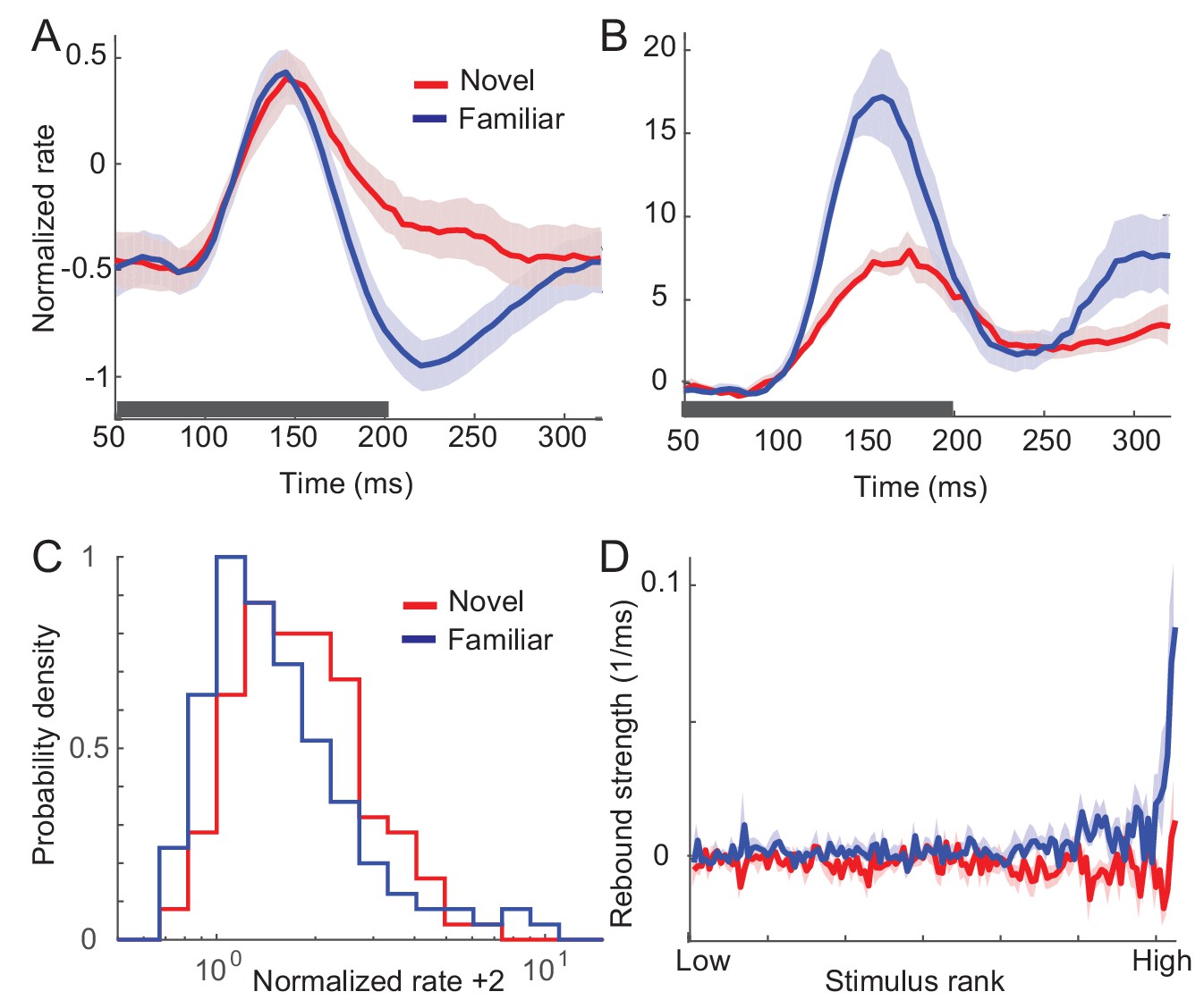
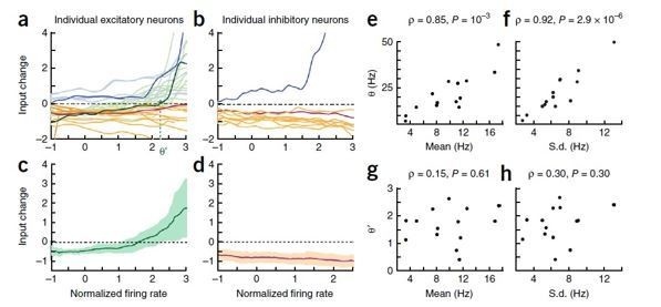
Changes in response dynamics of putative excitatory neurons with learning in a passive viewing task (Lim et al., 2015; Woloszyn and Sheinberg, 2012).

(A, B) Average and maximal response to familiar (blue) and novel (red) stimuli. For each excitatory neuron, we normalized firing rates by the mean and standard deviation of time-averaged activities over novel stimuli during stimulus presentation (80 ms-200 ms after the stimulus onset) and took the average over stimuli (A) and the response with the highest time-averaged activity (B). Solid curves are activities averaged over neurons, and shaded regions represent mean ± s.e.m of activities averaged over individual neurons. The gray horizontal bar represents the visual stimulation period starting at 0 ms. (C) Distribution of time-averaged activities during stimulus presentation. For each neuron, according to time-averaged activities, a stimulus was rank-ordered among familiar and novel stimuli, respectively. At each rank of the stimuli, we averaged the normalized response over neurons, and obtained the distributions of activities over different ranks of stimuli. To avoid negative values in the x-axis on a logarithmic scale, we added two to normalized rates. (D) Rebound strength of damped oscillation. At each rank of stimuli, the rebound strength was quantified by the slope of changes of activities between 230 ms and 320 ms after the stimulus onset.

https://doi.org/10.7554/eLife.44098.002

Figure 1—source code 1 Data for Figure 1D.: https://doi.org/10.7554/eLife.44098.019
Download elife-44098-fig1-code1-v2.m

Figure 1—figure supplement 1

Download asset Open asset

Changes in response dynamics of putative inhibitory neurons with learning in a passive viewing task (Woloszyn and Sheinberg, 2012).

(A, B) Average (A) and maximal (B) response to familiar (blue) and novel (red) stimuli. (C) Distributions of time-averaged activities. (D) Rebound strengths in inhibitory neurons before and after learning. Activities and rebound strengths were quantified in the same manner as in the excitatory neurons in Figure 1.

https://doi.org/10.7554/eLife.44098.003

Figure 2

Download asset Open asset

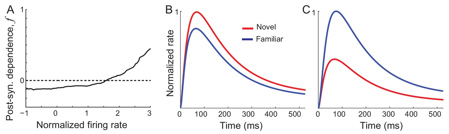
Networks with synaptic plasticity in recurrent connections without slow negative feedback.

(A) Example post-synaptic dependence of recurrent synaptic plasticity inferred from changes of time-averaged responses. Dependence of synaptic plasticity on the post-synaptic rate, f in Equation (2), shows depression for low rates and potentiation at high rates. (B, C) Average (B) and maximal (C) response before (red) and after (blue) learning for the network with synaptic plasticity only in recurrent connections.

https://doi.org/10.7554/eLife.44098.004

Figure 3 with 2 supplements

Download asset Open asset

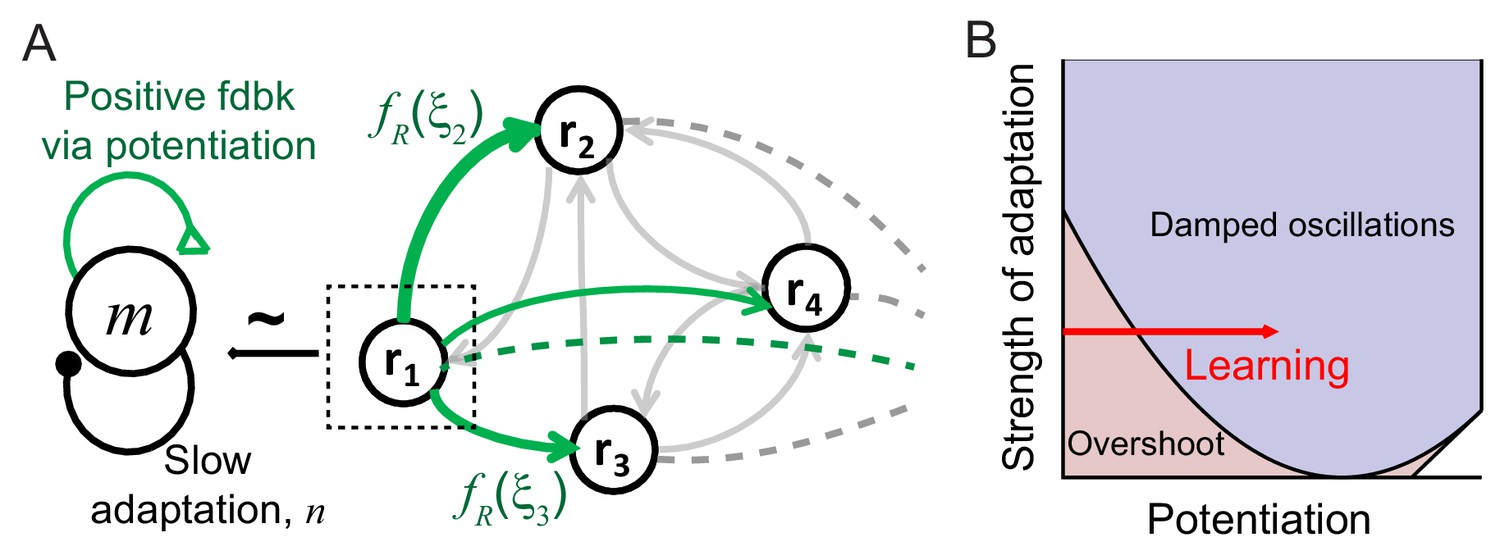
Mechanism of generating damped oscillations after learning.

(A) Schematics of the dynamics after learning. The overlap variable m is similar to activities of high rate neurons represented as r₁, and n represents adaptation in m. These high rate neurons drive a damped oscillation in the remaining population whose strength is proportional to the post-synaptic dependence of recurrent synaptic plasticity $f_{R} (ξ_{i})$ . (B) Interactions between potentiation of recurrent inputs and a slow adaptation mechanism. The strength of potentiation is proportional to ${\bar{f g}}_{R}$ (Equation 4) which is 0 before learning. The separatrix dividing overshoot and damped oscillations is shown as a parabola defined by ${\bar{f g}}_{R}$ , the strength of adaptation k and time constants τ_R and τ_A.

https://doi.org/10.7554/eLife.44098.005

Figure 3—figure supplement 1

Download asset Open asset

Networks with synaptic plasticity only in recurrent connections with slow negative feedback.

Average (A,C) and maximal (B,D) response before (red) and after (red) learning with potentiation-dominant (A,B) or depression-dominant (C,D) synaptic plasticity rules. The simulation of the mean-field dynamics is the same as in Figure 5 with the same parameters except ${\bar{f}}_{F} = 0$ , ${\bar{f}}_{R} = 0.1$ (A,B), and ${\bar{f}}_{R} = - 0.2$ (C,D).

https://doi.org/10.7554/eLife.44098.006

Figure 3—figure supplement 2

Download asset Open asset

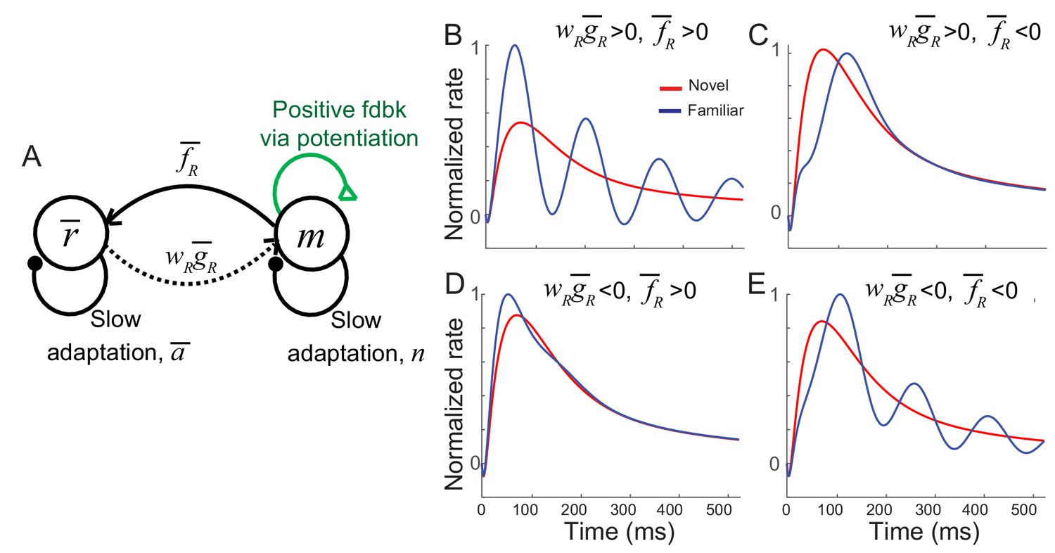
Networks with synaptic plasticity only in recurrent connections without the constraint of the sum normalization of synaptic weights achieved by $\sum g_{k} (ξ_{j}) = 0$ .

(A) Schematics of the mean-field dynamics after learning. The qualitative difference between the dynamics with or without the constraint is the feedback from $\bar{r}$ to m (dotted curve). (B–E) Average response before (red) and after (blue) learning with different ${\bar{f}}_{R}$ and $w_{R} {\bar{g}}_{R}$ . As the case with the constraint, the oscillation can be generated by the strong positive feedback and slow negative feedback in the m dynamics, and the synchronous oscillations in $\bar{r}$ and m are determined by the signs of ${\bar{f}}_{R}$ and $w_{R} {\bar{g}}_{R}$ . When ${\bar{f}}_{R}$ and $w_{R} {\bar{g}}_{R}$ have the same signs, a positive feedback loop through $\bar{r}$ further boosts the oscillation in the m dynamics (B,E), while the opposite signs of ${\bar{f}}_{R}$ and $w_{R} {\bar{g}}_{R}$ suppress the oscillation (C,D). Synchrony oscillation between $\bar{r}$ and m requires ${\bar{f}}_{R}$ >0 (B,D), and $w_{R} {\bar{g}}_{R}$ >0 further increase overall oscillation as well as average rates (B). On the other hand, $w_{R} {\bar{g}}_{R}$ <0 diminishes the oscillation while decreasing average rates (D). None of these cases can reproduce the experimental observations, synchronous oscillations in $\bar{r}$ and m with a decrease in the average rates. Thus, additional changes as the feedforward synaptic plasticity are still required without the constraint on the pre-synaptic dependence. The simulation of the mean-field dynamics is the same as in Figure 3—figure supplement 1 except w_R = −0.1, a = −6.5, b = 5.5, t₀ = 400 ms, t₁ = 40 ms, ${\bar{f}}_{R}$ =±0.1 and $w_{R} {\bar{g}}_{R}$ =±1.

https://doi.org/10.7554/eLife.44098.007

Figure 4

Download asset Open asset

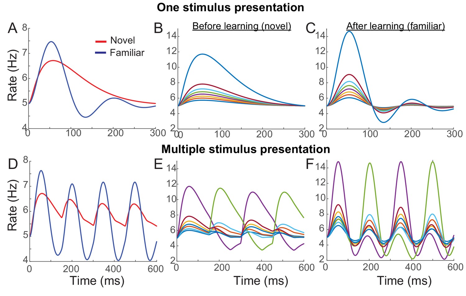
Example network reproducing the effects of visual learning in one stimulus presentation (A–C) and successive presentation of two stimuli (D–F).

The network implements potentiation in the recurrent connections through Hebbian synaptic plasticity, depression in the feedforward connections through uniform scaling down of the external inputs, and spike-adaptation mechanisms. Mean responses reproduce the effects of visual learning predicted in the mean-field dynamics, showing average reduction and stronger oscillations (A, D). Representative individual activities before (B,E) and after (C,F) learning show that activities in neurons with high firing rates increase with strong oscillation after learning (E,F), but the rank of stimuli is shuffled with the arrival of a new stimulus.

https://doi.org/10.7554/eLife.44098.008

Figure 4—source code 1 MATLAB code for Figure 4.: https://doi.org/10.7554/eLife.44098.020
Download elife-44098-fig4-code1-v2.m

Figure 5 with 3 supplements

Download asset Open asset

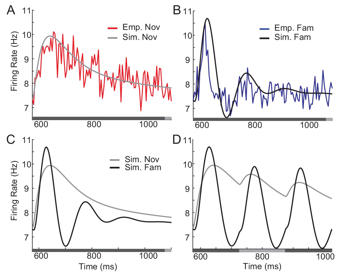
Comparison between network simulation and data obtained in a dimming-detection task.

(A, B) Fitting response dynamics (red in A and blue in B) using mean-field equations (gray in A and black in B) for novel (A) and familiar (B) stimuli. (C,D) Simulation for one stimulus presentation (C) and successive presentation of stimuli (D). The gray horizontal bar represents the visual stimulation period starting at 500 ms and x-axis is truncated to show activities from their onsets. In A-C, the stimulus was presented for a duration that was a sum of a fixed duration (650 ms shown in the dark gray) and a random duration (shown in the light gray). In D, different gray bars represent different stimuli shown alternatively for a duration of 150 ms.

https://doi.org/10.7554/eLife.44098.009

Figure 5—source code 1 Data for Figure 5.: https://doi.org/10.7554/eLife.44098.021
Download elife-44098-fig5-code1-v2.mat
Figure 5—source code 2 MATLAB code for Figure 5.: https://doi.org/10.7554/eLife.44098.022
Download elife-44098-fig5-code2-v2.m

Figure 5—figure supplement 1

Download asset Open asset

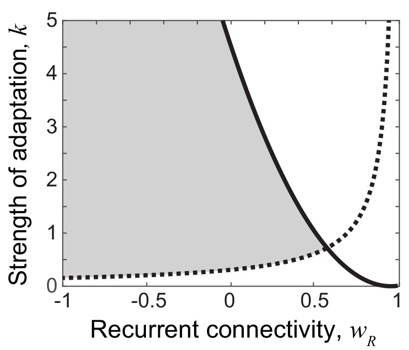
Constraints on w_R and k to reproduce responses to novel stimuli (shaded area).

In the dynamics of $\bar{r}$ and $\bar{a}$ in Equation (4), no damped oscillation for novel stimuli provides a constraint $k \leq {((- 1 + w_{R}) / τ_{R} + 1 / τ_{A})}^{2} τ_{R} τ_{A} / 4$ (solid black line). To analytically obtain the constraints for the lower peak in the successive presentation of novel stimuli, we assumed that during the rising phase of activity, adaptation variable and external inputs are constant. Also, we assumed neural activity changes linearly during the rising and decaying phase. Under these assumptions, the lower peak for the second novel stimuli provides the constraint $c (τ_{R}, τ_{A}, t_{0}, t_{1}, r_{1} / r_{0}) < (1 - w_{R}) k$ (the dotted line). Here, c is a constant determined by time constants τ’s and t₀ and t₁ that are the durations of the rising and decaying phases, and r₀ and r₁ that are the activities at the end of the rising and decaying phases such that $c = \frac{r_{1} / r_{0} \cdot τ_{R} / t_{0}}{1 - \exp (- t_{1} / τ_{A}) - (1 - r_{1} / r_{0}) (τ_{A} / t_{0} (\exp (- t_{1} / τ_{A}) - 1) + 1)}$ . The parameters used in this figure are τ_R = 5 ms, τ_A = 200 ms, t₀ = 30 ms, t₁ = 120 ms, r₁/r₀ = 0.7.

https://doi.org/10.7554/eLife.44098.010

Figure 5—figure supplement 2

Download asset Open asset

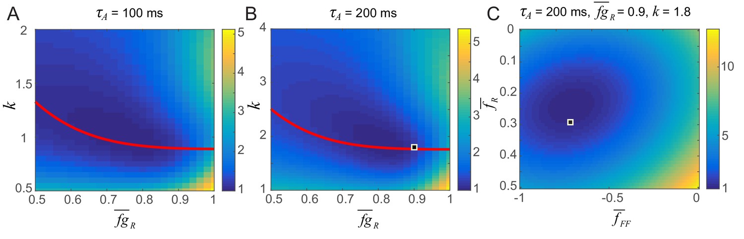
Parameter search for the strengths of potentiation and adaptation (A,B) and average post-synaptic dependence of recurrent and feedforward connections, ${\bar{f}}_{R}$ , and ${\bar{f}}_{F}$ (C).

The color map shows the distance between the data and simulation of the response for familiar stimuli normalized by the lowest distance. The red curve in A and B shows the pairs of ${\bar{f g}}_{R}$ and k that provide the damped oscillation with its period around 150 ms and provide a good fit to the data. In Figure 5, we chose ( ${\bar{f g}}_{R}$ ,k) = (0.9,1.8) (the square in B) and ( ${\bar{f}}_{R}$ , ${\bar{f}}_{F}$ ) = (0.3,–0.7) (the square in C) for τ_A = 200 ms which gives a good fit to a data in a dimming detection task (Figure 5B) as well as generating strong resonance behavior in the successive stimulus presentation (Figure 5D). The distance between the data and simulation is obtained by comparing them between 0 and 300 ms after the activity onset except between 50 ms and 100 ms due to the rapid decrease of activity between 50 and 100 ms which cannot be captured by the simulation.

https://doi.org/10.7554/eLife.44098.011

Figure 5—figure supplement 3

Download asset Open asset

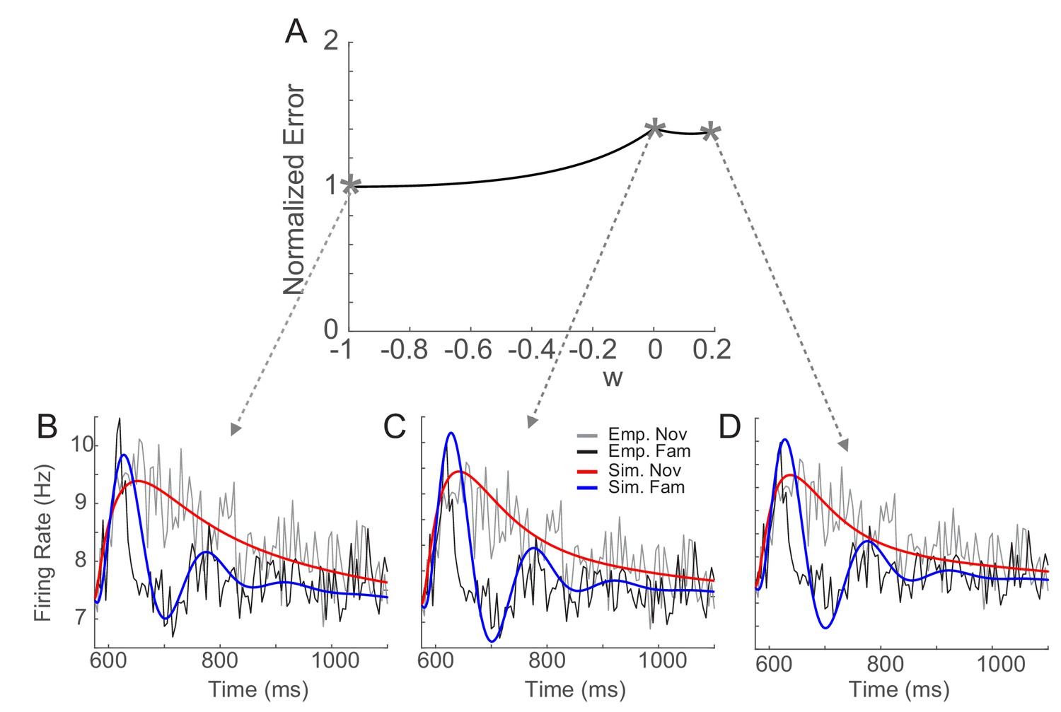
Sensitivity of fitting to changes in the recurrent connectivity strength before learning, w_R.

(A) The distance between the data and simulation of the response for familiar stimuli normalized by the lowest distance as in Figure 5—figure supplement 2. (B–D) Comparison between the data and network simulations for different w_R. For a wide range of w_R, the simulation fit the data well. The parameters are the same as in those in Figure 5 except a, b, t₀, and t₁ which were adjusted for each w_R to reproduce response to novel stimuli.

https://doi.org/10.7554/eLife.44098.012

Figure 6 with 3 supplements

Download asset Open asset

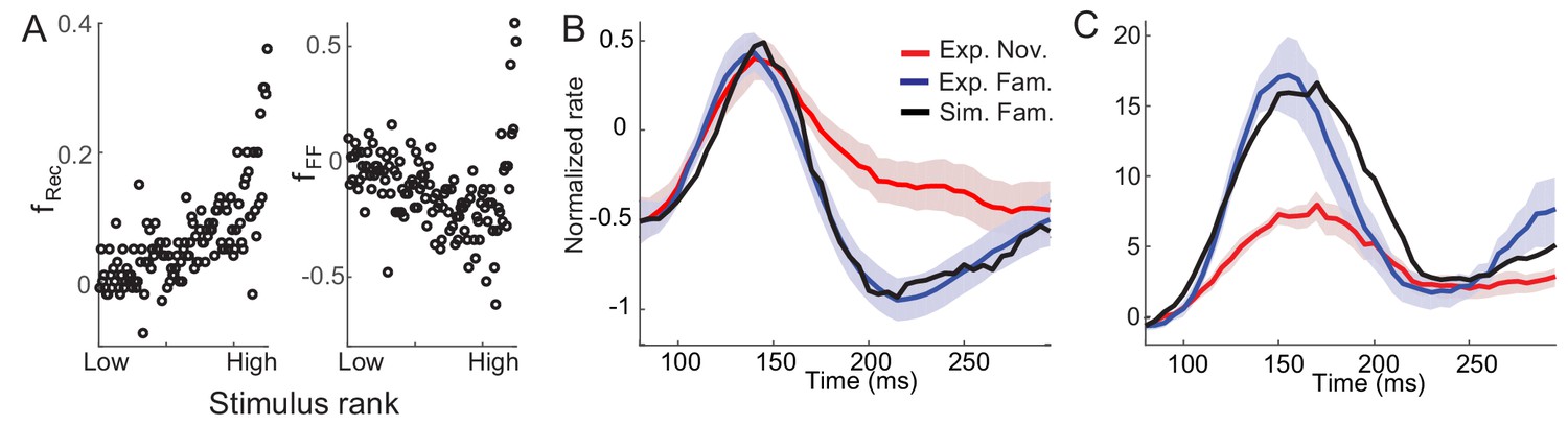
Post-synaptic dependence of synaptic plasticity in recurrent (left) and feedforward (right) connections derived from a passive viewing task (A) and comparison between the data and network simulations for average (B) and maximal (C) responses.

The external inputs were chosen so that the response to novel stimuli is the same in the experiment and simulation (red in B,C). With the derived post-synaptic dependence in the recurrent and feedforward connections (A), the response to familiar stimuli was simulated (black in B,C).

https://doi.org/10.7554/eLife.44098.013

Figure 6—source code 1 MATLAB code for Figure 6.: https://doi.org/10.7554/eLife.44098.023
Download elife-44098-fig6-code1-v2.m

Figure 6—figure supplement 1

Download asset Open asset

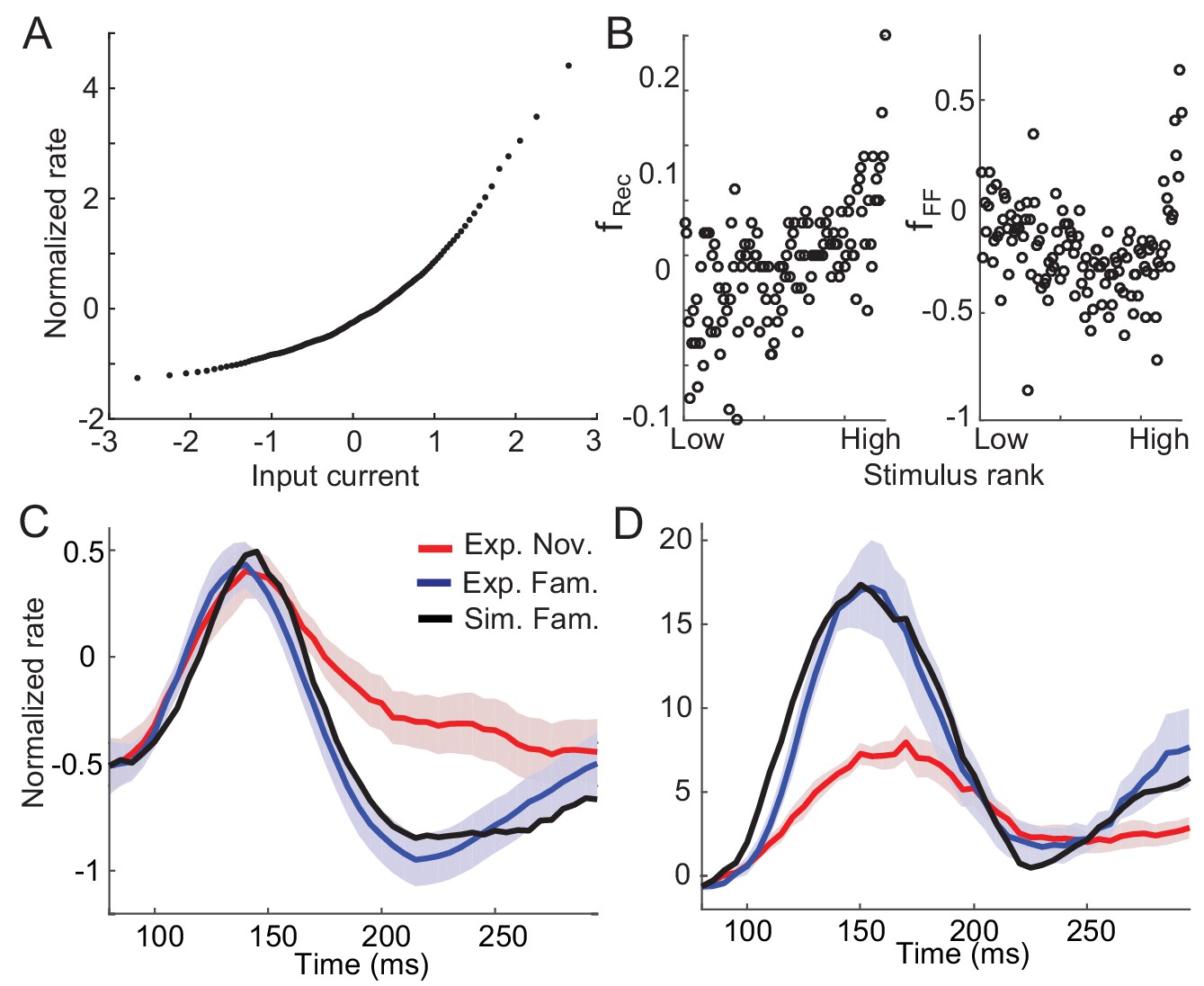
Example nonlinearity in dynamics and synaptic plasticity inferred under nonlinearity.

(A) Nonlinear input current-output firing rate transfer function that leads to nonlinear dynamics in the circuits. Under the assumptions of a normal distribution of input currents before learning and monotonically increasing transfer function, the transfer function was obtained from the distribution of time-averaged responses to novel stimuli (Lim et al., 2015). (B) Post-synaptic dependence of synaptic plasticity in the recurrent (left) and feedforward (right) connections that best fit the changes in response dynamics with the nonlinear transfer function in (A). (C,D) Comparison between data and network simulations for average (C) and maximal responses (D) (blue for data and black for network simulation).

https://doi.org/10.7554/eLife.44098.014

Figure 6—figure supplement 2

Download asset Open asset

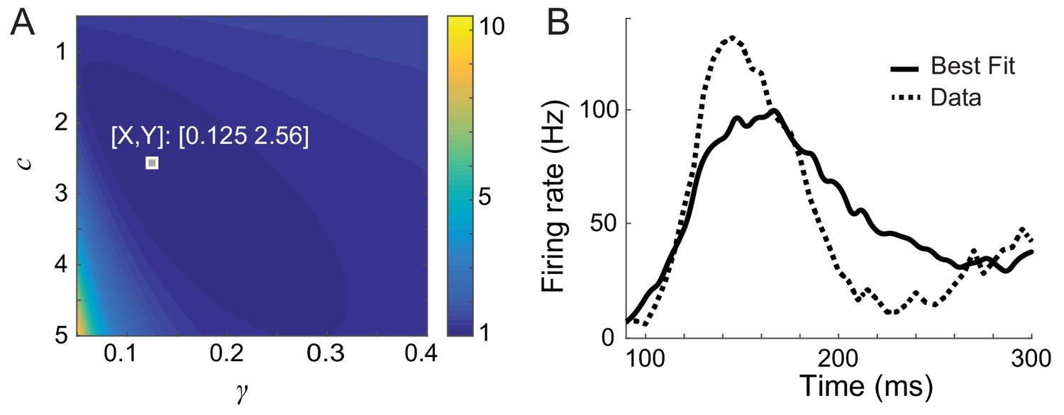
Short-term depression cannot reproduce a damped oscillation after learning.

(A) Parameter search of the strength of depression (γ) and strength of potentiation (c = $f_{m}^{R} g_{m}^{R}$ ). The color map shows the distance between the data and simulation of the response for familiar stimuli normalized by the lowest distance. (B) Time course of the response to the best familiar stimuli with the best-fitted parameters γ = 0.125, and $f_{m}^{R} g_{m}^{R}$ = 2.56. Other parameters are $τ_{R}$ = 5 ms, $τ_{x}$ = 200 ms, and $I_{m}^{X}$ is obtained from the response to the best novel stimuli.

https://doi.org/10.7554/eLife.44098.015

Figure 6—figure supplement 3

Download asset Open asset

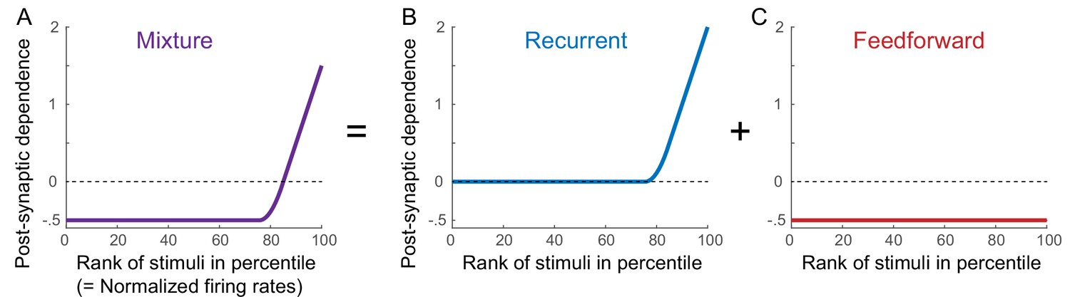
Schematics of synaptic plasticity rules in different connections.

The learning rule inferred from time-averaged activities (A) can be considered to be a combination of recurrent (B) and feedforward (C) synaptic plasticity. Such a learning rule shows a similar dependence on the normalized rates (equivalently the rank of stimuli) across different neurons (A; Lim et al., 2015). Inspired by this, we assumed the same synaptic plasticity rules of recurrent and feedforward connections across different neurons for normalized firing rates (B,C).

https://doi.org/10.7554/eLife.44098.016

Figure 7

Download asset Open asset

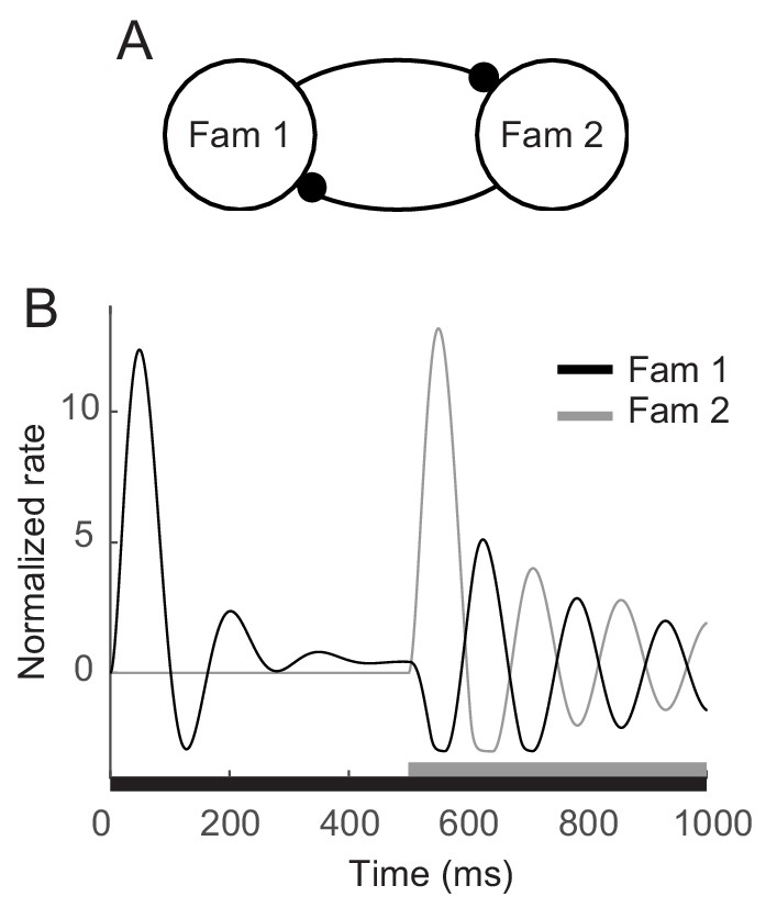
Enhanced oscillation through competitive interactions between different stimuli.

(A) Two mutually inhibitory populations selectively responding to stimuli 1 and 2, respectively. The dynamics of each population follows the dynamics of m in the mean-field description for a single familiar stimulus in Figures 3A,5. (B) Time course of visual responses of two populations with different stimulus onsets (black and gray bars below). Stimulus 2 was present 500 ms after the onset of stimulus 1, and the population two was assumed to be silent before the arrival of stimulus 2. After the onset of stimulus 2, visual response selective to stimulus one was transiently suppressed and showed stronger oscillation compared to that under the single stimulus presentation.

https://doi.org/10.7554/eLife.44098.017

Author response image 1

Download asset Open asset

Additional files

Source code 1 Data for Figures 1 and 6.: https://doi.org/10.7554/eLife.44098.018
Download elife-44098-code1-v2.mat
Transparent reporting form: https://doi.org/10.7554/eLife.44098.024
Download elife-44098-transrepform-v2.docx

Download links

A two-part list of links to download the article, or parts of the article, in various formats.

Downloads (link to download the article as PDF)

Open citations (links to open the citations from this article in various online reference manager services)

Mendeley

Cite this article (links to download the citations from this article in formats compatible with various reference manager tools)

Sukbin Lim

(2019)

Mechanisms underlying sharpening of visual response dynamics with familiarity

eLife 8:e44098.

https://doi.org/10.7554/eLife.44098

Sign up for email alerts

Privacy notice