Fixation-pattern similarity analysis reveals adaptive changes in face-viewing strategies following aversive learning
- University Medical Center Hamburg-Eppendorf, Germany
Figures
Figure 1 with 2 supplements
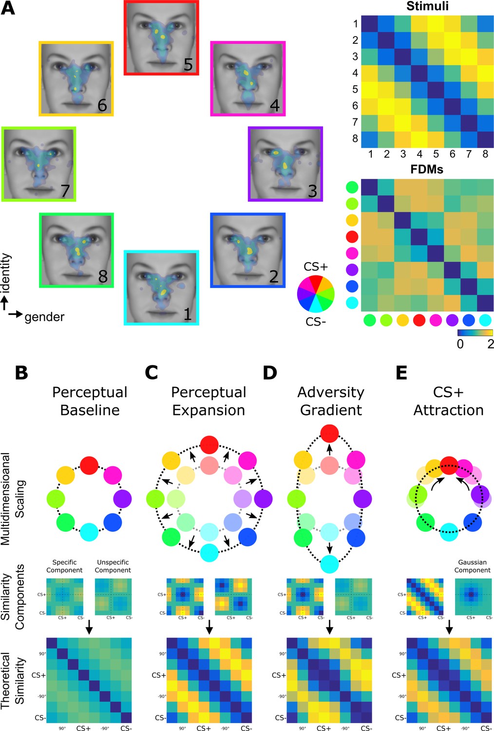
Fixation-pattern similarity analysis.
(A) eight exploration patterns (colored frames) from a representative individual overlaid on eight face stimuli (1 to 8) calibrated to span a circular similarity continuum across gender and identity dimensions. A pair of maximally dissimilar faces was randomly selected as CS+ (red) and CS– (cyan; see color wheel). Similarity between the eight faces was calibrated to have a perfect circular organization with lowest dissimilarity (blue) between neighbors, and highest dissimilarity (yellow) for opposing pairs. FPSA summarizes the similarity relationship between the eight exploration patterns as a symmetric 8 × 8 matrix (bottom right panel). 4th and 8th columns (and rows) are aligned with the CS+ and CS–, respectively. (B–E) Multidimensional scaling representation of four theoretical similarity relationships investigated with FPSA (top row). Each colored node represents one exploration pattern (red: CS+; cyan: CS–), where internode distances are proportional their dissimilarity (bottom row). Shaded nodes in (C–E) depict the pre-learning state in (B). Dissimilarity matrices are further decomposed onto basic similarity components (middle row) centered either on the CS+/CS– (specific component) or +90°/–90° faces (unspecific component). A third component shown in (E) is uniquely centered on the CS+ face (Gaussian component). In (B), equal contribution of basic components results in circularly similar exploration patterns. In (C), a stronger equal contribution results in a better global separation of all exploration patterns, that is expansion (denoted by radial arrows). In (D), a stronger contribution of the specific component results in a biased separation of exploration patterns specifically along the adversity gradient defined between the CS+ and CS– nodes. In (E), the Gaussian component centered on the CS+ face can specifically decrease the dissimilarity of exploration patterns for faces similar to the CS+, resulting in circularly shifted nodes (circular arrows) while preserving the global circularity of the similarity relationships.
Figure 1—figure supplement 1
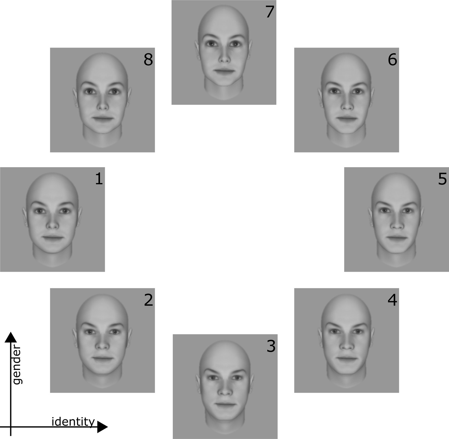
Face stimuli.
Set of 8 faces that were calibrated to form a circular similarity continuum. Faces vary along the two dimensions of gender (vertical axis) and identity (horizontal axis). See Figure 1—figure supplement 2 for the calibration process.
Figure 1—figure supplement 2
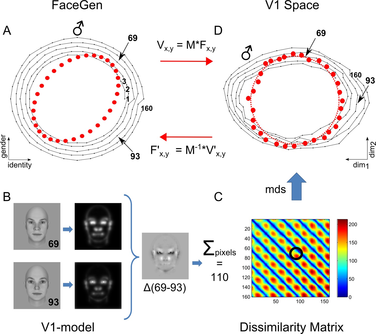
Calibration of faces using a simple V1 model tuned to human psychophysics.
(A) Using the FaceGen software, 160 faces forming five concentric circles were generated with coordinates varying in gender and identity dimensions (connected black dots in the left panel). Maximally male faces are located at 12 o’clock direction and indicated with the male symbol. (B) V1 representations of faces were modeled according to Yue et al. (2012). This is illustrated for faces 69 and 93. The difference between these two faces resulted in a Euclidean distance of 110. The pair-wise Euclidean distance for all the 160 faces are shown in (C) as a dissimilarity matrix. The resulting dissimilarity matrix exhibits five major bands corresponding to five concentric circles. By applying MDS, we obtained the representational space of V1 shown in (A, right panel). Note that the most male face is 45° counter-clockwise rotated with respect to the main axes of in V1 representation. The mapping between FaceGen coordinates and V1 representational space thus involved a rotation and scaling which was captured by the matrix M. We therefore used the inverse of M, to achieve coordinates of perfect circularity based on this V1 model. This ensured that faces along the similarity continuum were characterized by controlled changes for every angular step based on the model used.
Figure 2
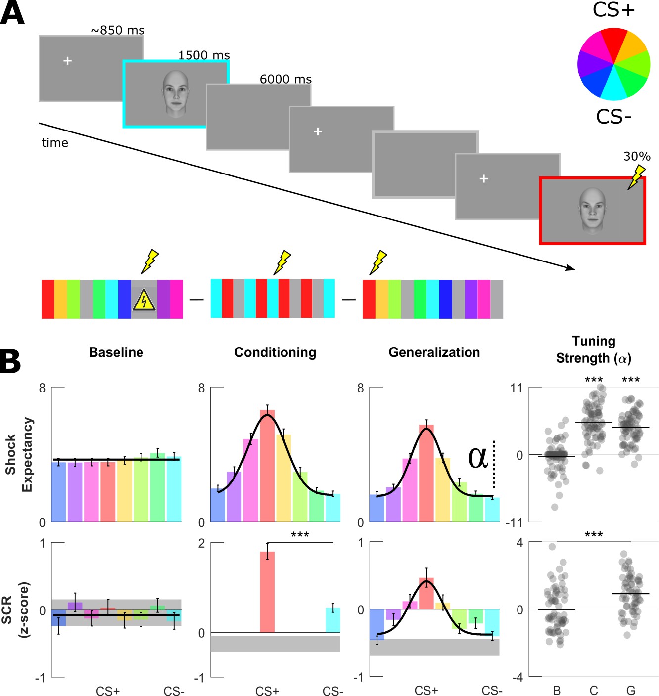
Aversive learning procedure and univariate generalization profiles.
(A) On every trial, one randomly selected face was presented for 1.5 s preceded by a fixation cross placed outside of the face on either the left or right side. In null trials, no face was shown (gray frame) resulting in a SOA of ~6 or~12 s. For each volunteer, a pair of most dissimilar faces was randomly selected as the CS+ (red) and CS– (cyan, see color wheel). During baseline, UCSs (shock sign) were completely predictable by the presentation of a triangular signboard. During conditioning and generalization, the CS+ face was paired with an aversive outcome in ~30% of trials allowing recording of responses from non-reinforced CS+ trials. (B) Group-level fear-tuning based on subjective ratings of UCS expectancy (n = 74) and SCR (n = 63) for different phases. Responses are aligned to the CS+ of each volunteer separately (errorbars: SEM across subjects). Black horizontal lines or curves indicate the winning model (p<0.001, log-likelihood ratio test), that is horizontal null model or the Gaussian model. Gray shaded areas in SCR depict response amplitudes evoked by null trials (mean and 95% CI). Scatter plots show amplitude parameter of Gaussian fits (denoted by alpha symbol) for each volunteer. Horizontal lines within the scatterplots depict group-level means, asterisks indicate significant differences in α (compared to baseline phase, paired t-test, ***: p<0.001).
Figure 3 with 3 supplements
Fixation-pattern similarity analysis.
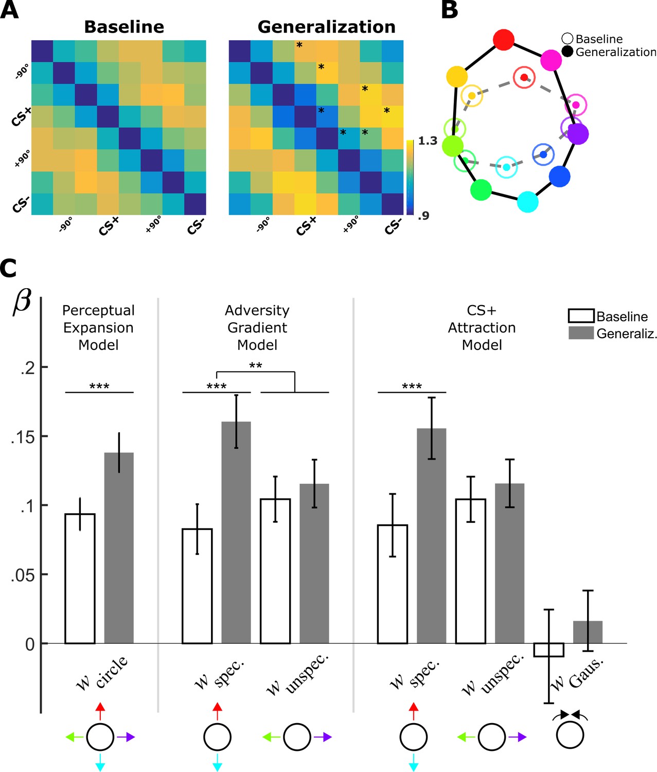
(A) Dissimilarity matrices of exploration patterns for baseline (left panel) and generalization phases (right panel). Fourth and eight columns (and rows) are aligned with each volunteer’s CS+ and CS– faces, respectively. Asterisks on the upper diagonal denote significant differences from the corresponding element in baseline. (B) Two-dimensional multidimensional scaling method used for visualization of the 16 × 16 dissimilarity matrix (not shown) comprising baseline and generalization phases. Distances between nodes are proportional to the dissimilarity between corresponding FDMs (open circles: baseline; filled circles: generalization phase; same color scheme as in Figure 1). (C) Bar plots (M ± SEM) depict predictor weights estimated for single-participants before (white bars) and after (gray bars) aversive learning (Left: Perceptual Expansion Model; Middle: Adversity Gradient Model; Right: CS+ Attraction Model). wcircle: weight for the circular component, which is the sum of equally weighted specific and unspecific components; wspecific/wunspecific: weights for specific and unspecific components; wGauss: weight for Gaussian component centered uniquely on the CS+. (**: p<0.01; ***: p<0.001, paired t-test).
Figure 3—figure supplement 1
Correlation between FPSA anisotropy and tuning strength.
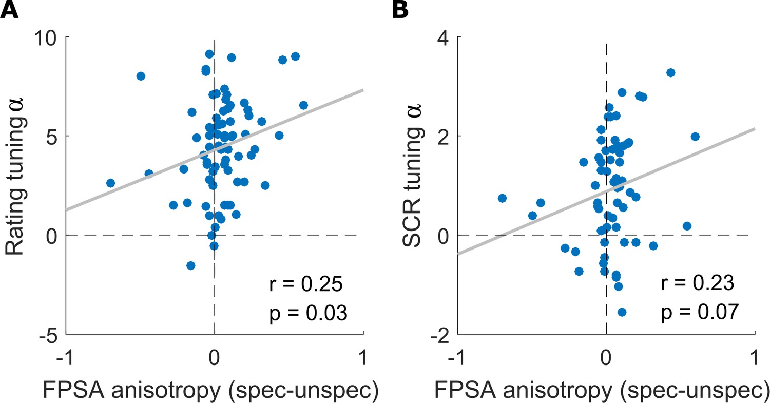
Correlation between single subject’s model parameters from the winning Adversity Gradient model and (a) behavioral (rating) and (b) autonomous (SCR) outcomes. FPSA anisotropy in the individual fixation pattern is the difference between the specific and the unspecific component, that is higher values correspond to stronger ellipsoidness along the specific dimension within one individual. The tuning strength is given by the amplitude parameter α of the Gaussian fit on the respective outcome (cf. amplitude parameters in Figure 2B). The gray line depicts the least-squares fit line.
Figure 3—figure supplement 2
Model parameters for Adversity Gradient Model across subsequent test runs.
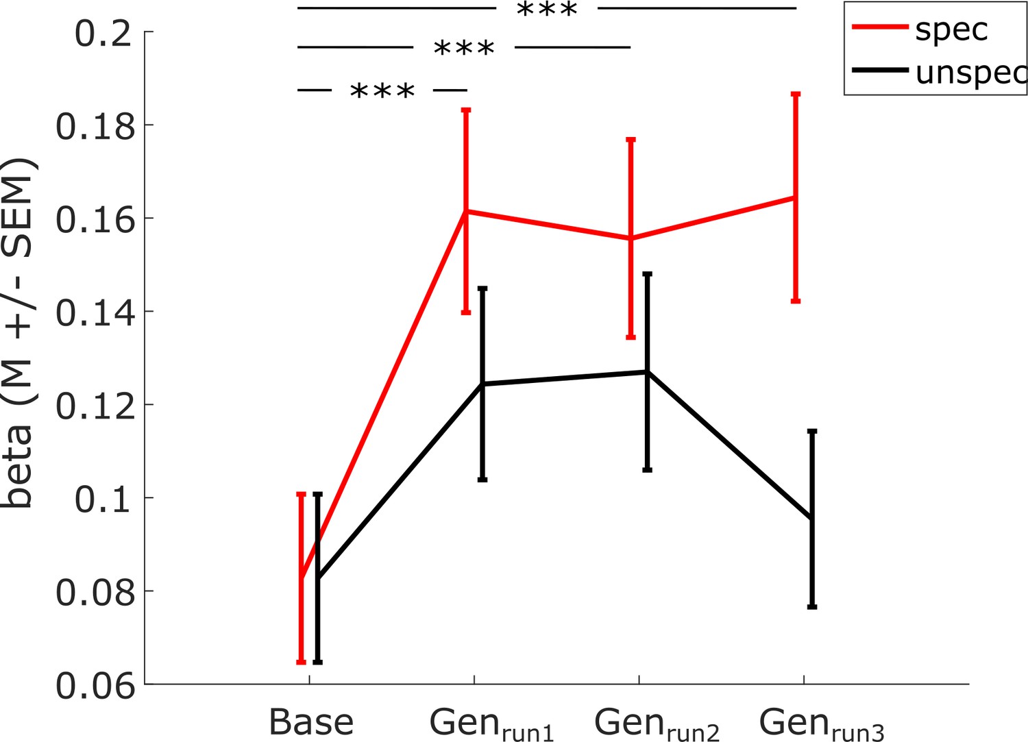
Beta estimates from the Adversity Gradient model of the specific and unspecific component when modeling data from the three generalization phase (‘Gen’) runs independently. The model estimates were computed on single subject dissimilarity matrices (cf. Figure 1). Shown is the average weight for the whole group, error bars indicate the SEM across subjects. Asterisks indicate significant differences of beta estimates of single generalization run compared to baseline phase (paired t-tests, ***: pcorr <0.001), showing that the unspecific component did not increase significantly from baseline to any of the generalization runs. Results of a repeated measures ANOVA (experimental run ×predictor (spec/unspec)): main effect of predictor (F(1, 73)=3.8, p=0.056, interaction of predictor (spec/unspec) with experimental run F(1,73) = 2.6, p=0.054).
Figure 3—figure supplement 3
Gaussian Mixture Models on individual anisotropy effects.
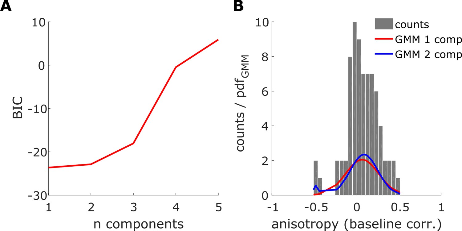
(A) Bayesian Information Criterion (BIC) for Gaussian Mixture Model (GMM) of n components based on single subject anisotropy values (baseline corrected, that is (wspecific_gen-wunspecific_gen) – (wspecific_base-wunspecific_base)). (B) Histogram of single subject anisotropy values (same as in A). Lines represent probability density functions of the resulting Gaussian distributions of the GMM on n = 1 (red, ‘GMM1’) and n = 2 (blue, ‘GMM2’) components, which are shown in detail as these models resulted in the lowest BIC (BICGMM1 = −23.7, BICGMM2 = −22.9). As visible, GMM1 resulted in one component centered on μ = 0.07, while GMM2 resulted in two Gaussians centered on μ1 = −0.48 = and μ2 = 0.09 with mixing proportions mp1 = 0.04 and mp2 = 0.96.
Figure 4 with 1 supplement

Classification of FDMs using support vector machines.
(A) Classification of single trial FDMs using support vector machines. Before training, single FDMs of CS+ and CS- trials were reduced in their dimensionality (pixels) by a principal component analysis (PCA), resulting in a new representation in this feature space (red and cyan dots). A SVM was then trained to decode CS+ from CS- trials by finding a multidimensional hyperplane (dotted lines) separating CS+ from CS- patterns. The same was repeated for stimuli from the unspecific dimension (not shown). (B) Accuracy of SVM classification along the specific and unspecific dimension, trained within- subject for baseline (white) and generalization phase (gray) (M ± SEM, ***: t(73) = 4.8, p<0.001, *: t(73) = 2.1, p<0.05 paired t-test) (see Source code 1) (C) Activation patterns derived from hyperplanes of classification of CS+ vs CS- trials as shown in (A). Activation patterns were z-scored and averaged across subjects with the same underlying physical CS+ facei (ni = [10, 12, 8, 10, 8, 10, 8, 8]), then superimposed on the respective face stimulus (see Source code 1).
Figure 4—figure supplement 1
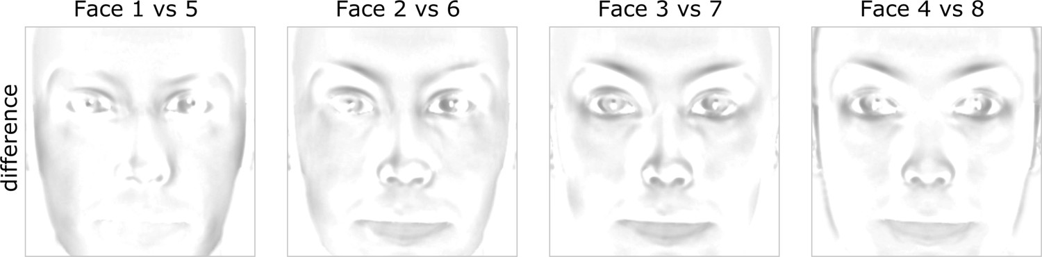
Physical differences in opposing faces.
Difference maps for each pair of opposing faces taken from the circular similarity continuum shown in Figure 1—figure supplement 1. For visualization purposes difference maps were inverted so that darker shades indicate stronger differences.
Figure 5 with 2 supplements
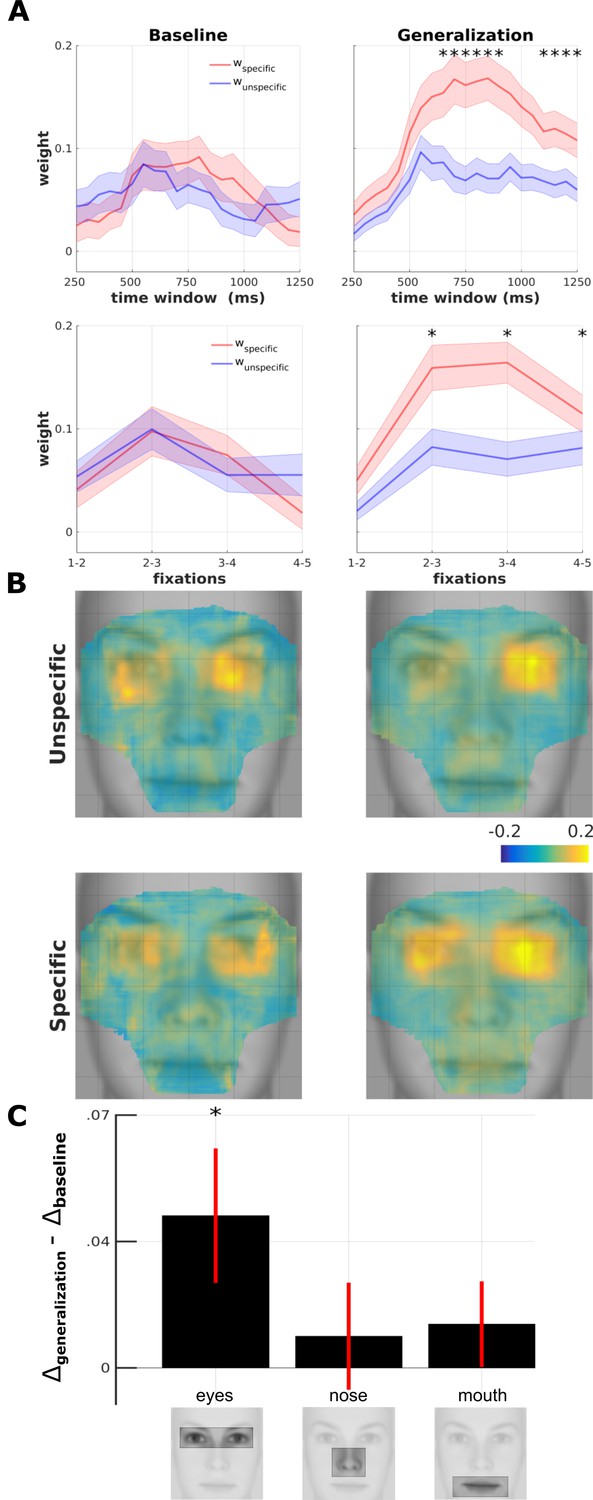
Spatio-temporal fixation-pattern similarity analysis.
(A) Temporal development of adversity-specific and unspecific exploration strategies (n = 61). Parameters of the adversity categorization model (red: specific; blue: unspecific) are computed using a moving time window of 500 ms at intervals of 50 ms for baseline (left panels) and generalization phase (right panel). Numbers on the x-axis denote the center of the moving window. Second row depicts the same analysis with fixation points sorted by rank. Asterisks indicate time points with statistically significant interaction testing for difference in anisotropy (wspecific – wunspecific) between test vs. baseline (*: p<0.05; Shaded area: SEM) (B) Four maps resulting from the searchlight-FPSA on FDMs from before and after conditioning (left vs. right columns) and for unspecific and specific (top vs. bottom rows) model parameters overlaid on an average face. The map is masked to contain 90% of all fixation density. (C) Difference of anisoptropy between before and after aversive learning (generalization – baseline) for three different ROIs (*: p<0.01, paired t-test).
Figure 5—figure supplement 1
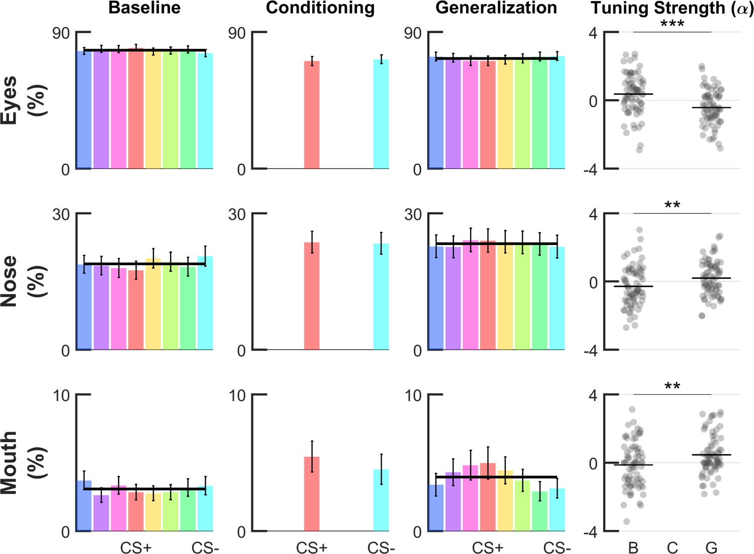
Generalization profiles on ROI-based fixation counts.
Group-level fear-tuning based on percentage of fixations in a given ROI (n = 74) for different phases. Fixation count data expressed as percentages are based on three major facial regions, that is eyes, nose and mouth (see Figure 5). Responses are aligned to the CS+ of each volunteer separately (errorbars: SEM across subjects) and normalized to a mask comprising the three ROIs. Black horizontal lines or curves indicate the winning model (p<0.001, log-likelihood ratio test), that is horizontal null model or the Gaussian model. In all situations, the null horizontal model was favored by the model comparison procedure. Scatter plots show amplitude parameter α of single-subject Gaussian fits. Horizontal lines within the scatterplots depict group-level means, asterisks indicate significant differences in α (compared to baseline phase, paired t-test, ***: p<0.001, **: p<0.01).
Figure 5—figure supplement 2
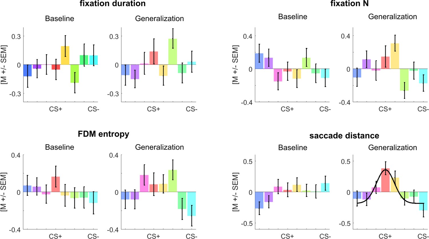
Generalization profiles of common fixation features.
Common fixation features, such as fixation duration, number of fixations (fixation N), saccade distance and average entropy in FDMs for baseline and generalization phase. Features were extracted from single trial FDMs, z-scored within subject and experimental phase, then averaged across participants. Error bars depict the SEM across subjects. The black horizontal curve indicates where features a significantly tuned to the CS+ (p<0.001, log-likelihood ratio test, Gaussian model vs. flat null-model).
Figure 6
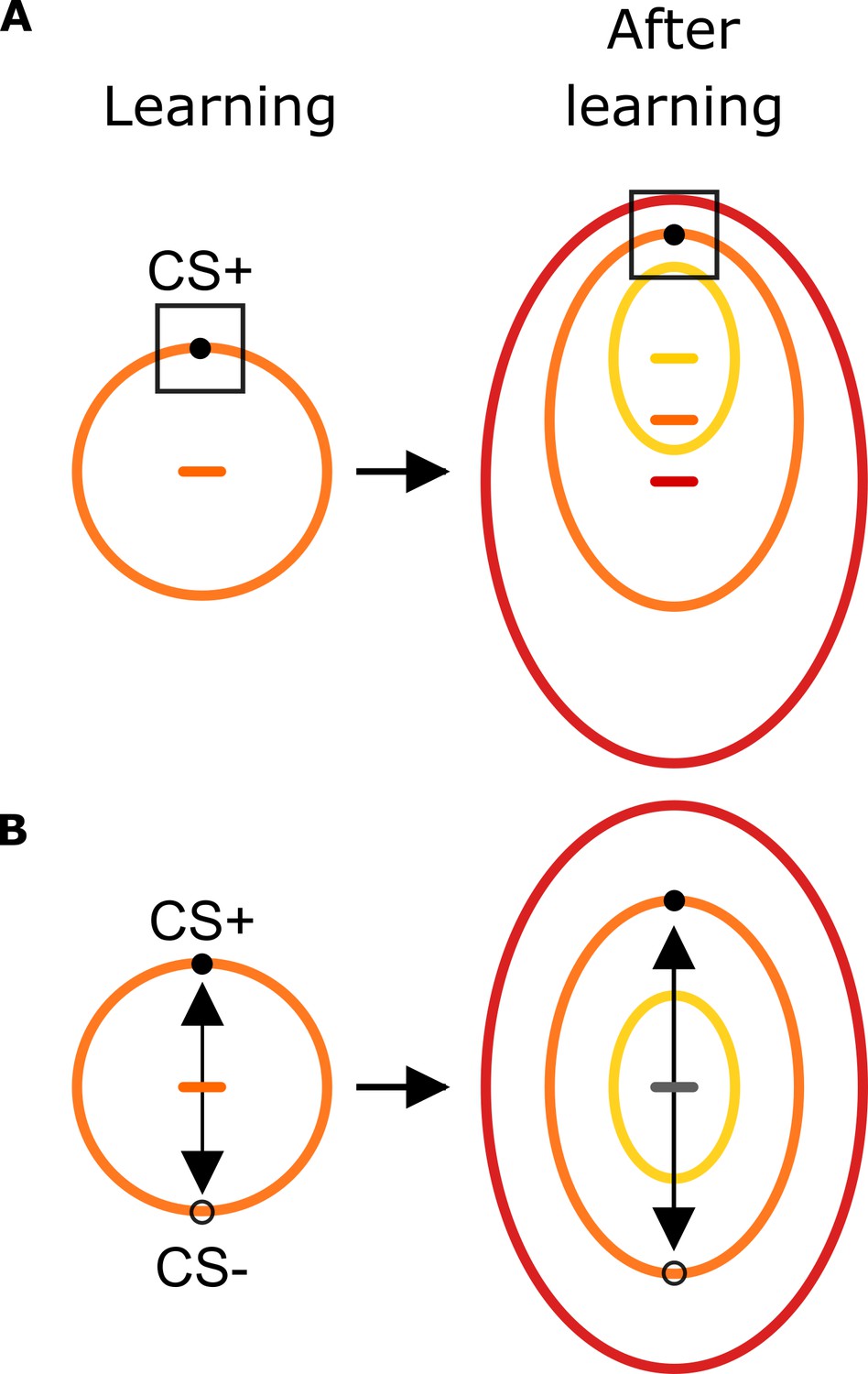
Predictions on the influence of aversive learning on sensory-motor foraging strategies.
Before learning, exploration strategies follow the circularity of the stimulus space (orange circle) in line with their presumed physical characteristics. (A) In one scenario, conditioning leads humans to learn the specific feature values that predict a harmful outcome (black square). When tested subsequently with stimuli organized as three concentric stimulus gradients, this scenario predicts faces that are similar to the CS+ face to be explored similarly. This results in a global shift in the center of gravity towards the CS+ face as indicated by yellow, orange and red horizontal dashes indicating the center of corresponding ellipses. (B) Humans learn the feature vector (black arrow) that best separates harmful and safety predicting stimuli. When tested with the concentric circular stimulus set, this scenario predicts three concentric ellipses sharing the same center of gravity (gray horizontal line).
Additional files
-
Source code 1
Code implementing classification of single trials with linear support vector machines (see Figure 4).
- https://doi.org/10.7554/eLife.44111.016
-
Supplementary file 1
Supplementary tables reporting mixed-effects modeling of the three models shown in Figure 1B–E.
(A) Mixed-effects modeling of the similarity matrices during the baseline phase with the Perceptual model shown in Figure 1B. (B) Mixed-effects modeling of the similarity matrices during the generalization phase with the Perceptual model shown in Figure 1B. (C) Mixed-effects modeling of the similarity matrices during the baseline phase with the Adversity Gradient model shown in Figure 1D. (D) Mixed-effects modeling of the similarity matrices during the generalization phase with the Adversity Gradient model shown in Figure 1D. (E) Mixed-effects modeling of the similarity matrices during the baseline phase with the CS+ Attraction model shown in Figure 1E. (F) Mixed-effects modeling of the similarity matrices during the generalization phase with the CS+ Attraction model shown in Figure 1E.
- https://doi.org/10.7554/eLife.44111.017
-
Transparent reporting form
- https://doi.org/10.7554/eLife.44111.018
Download links
A two-part list of links to download the article, or parts of the article, in various formats.
Downloads (link to download the article as PDF)
Open citations (links to open the citations from this article in various online reference manager services)
Cite this article (links to download the citations from this article in formats compatible with various reference manager tools)
Fixation-pattern similarity analysis reveals adaptive changes in face-viewing strategies following aversive learning
eLife 8:e44111.
https://doi.org/10.7554/eLife.44111


