Phylodynamic theory of persistence, extinction and speciation of rapidly adapting pathogens
- University of California, Santa Barbara, United States
- University of Basel, Swiss Institute for Bioinformatics, Switzerland
Figures
Figure 1
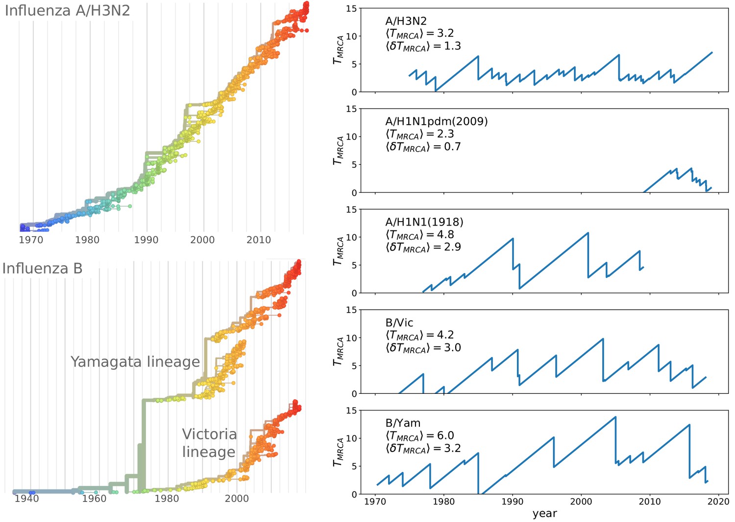
Spindly phylogenies and speciation in different human seasonal influenza virus lineages.
The top left panel shows a phylogeny of the HA segment of influenza A virus of subtype H3N2 from its emergence in 1968 to 2018. The virus population never accumulates much diversity but is rapidly evolving. The lower left panel shows a phylogeny of the HA segment of influenza B viruses from 1940 to 2018. In the 70s, the population split into two lineages known as Victoria (B/Vic) and Yamagata (B/Yam) in the 1970s. The graphs on the right quantify diversity via the time to the most recent common ancestor for different influenza virus lineages. Influenza B viruses harbor more genetic diversity than influenza A viruses. The subtype A/H3N2 in particular coalesces typically in 3y while deeps splits in excess of 5y are rare.
Figure 2

Viral populations escape adaptive immunity by accumulating antigenic mutations.
Via cross-reactivity, the immunity foot-print of ancestral variants (center of the graph) mediates competition between related emerging viral strains and can drive all but one of the competing lineages extinct. At high mutation rates and relatively short range of antigenic cross-reactivity, different viral lineages can escape inhibition and continue to evolve independently.
Figure 3 with 2 supplements
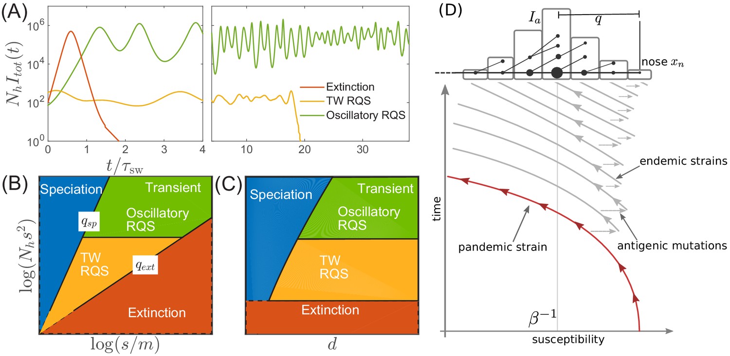
Extinction, speciation, and oscillations in multi-strain SIR models.
(A) Typical trajectories of infection prevalence in the parameter regimes corresponding to extinction (red), traveling wave RQS (yellow) and oscillatory RQS (green). Panels B and C schematically show parameter regimes corresponding to these qualitatively different behaviors. As explained in the text the boundaries of the RQS regime depend explicitly on the time scale considered (see also Figure 7). Simulation results supporting this diagram are shown in Figure 3—figure supplements 1 and 2. Panel (D) is a schematic illustrating how a novel pandemic strain (red) can settle into an endemic RQS state. As the cumulative number of infected individuals increases, the susceptible fraction decreases, and survival of the strain depends on the emergence of antigenic escape mutations (gray). The top part of the panel illustrates the population composition at a particular time point. Rare pioneering variants are mutations ahead of the dominant variant and grow with rate . (Note, that boundaries of the ‘extinction’ regime in (B,C) correspond to value close to one.) Different lineages are related via their phylogenetic tree embedded in the fitness distribution in the population.
Figure 3—figure supplement 1
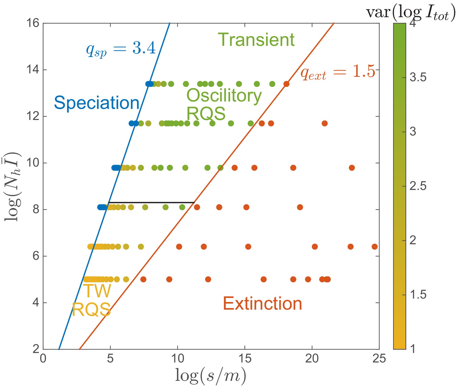
‘Phase diagram’ in the clone-based simulation.
The data points are assigned to phases using the following criteria. The extinction phase (red): ; The speciation phase (blue): ; The transient RQS regime (yellow and green): otherwise. Red and blue lines correspond to the extinction boundary and speciation boundary respectively, defined for . The black solid line corresponds to the onset of spontaneous oscillation . Color in the transient phase labels the amplitude of prevalence , increasing from yellow to green. Simulation set .
Figure 3—figure supplement 2

Value of across the ‘Phase diagram’.
This figure shows the same data as one with each data point colored by the corresponding value of , which is constant along the straight of different angle.
Figure 4 with 2 supplements
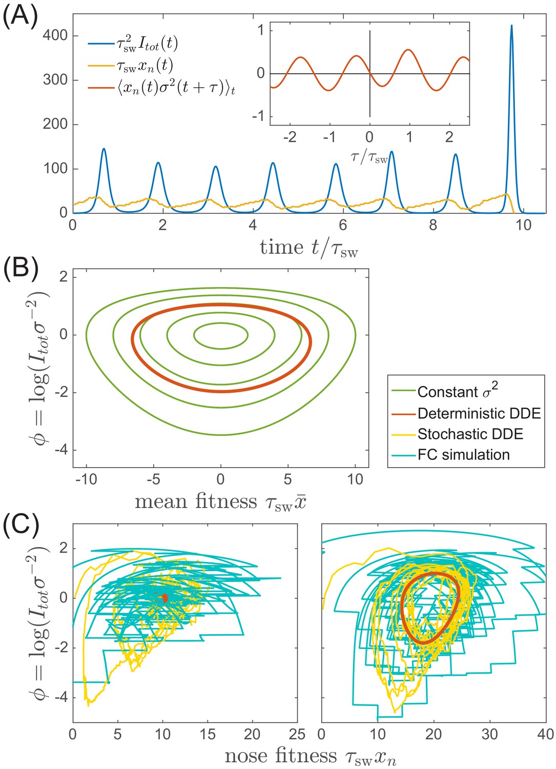
Oscillations in antigenically evolving populations.
(A) An example of the stochastic limit cycle trajectory from the fitness-class simulation. Note the rapid rise and fall of infection prevalence (blue), which causes a drop in nose fitness (yellow) which subsequently recovers (approximately linearly) during the remainder of the cycle. Fluctuations in and from cycle to cycle are caused by the stochasticity of , that is antigenic evolution in pioneer strains. A particularly large fluctuation about prior to the end, caused a large spike in prevalence, followed by the collapse of below zero and complete extinction. Inset (red) shows the cross-correlation between and which peaks with the delay (additional peaks reflect the oscillatory nature of the state and are displaced by integer multiples of mean period). (B) A family of limit cycles in the infection prevalence/mean fitness plane as described by Equation (11) with fixed variance. The variation of governed by the Equations 11 and 12 (in the deterministic limit) reduces the family to a single limit cycle (red); (C) Trajectories in the infection prevalence/nose fitness generated by the stochastic DD system in the regime above (right panel) and below (left panel) the oscillatory instability of the deterministic DD system.
Figure 4—figure supplement 1
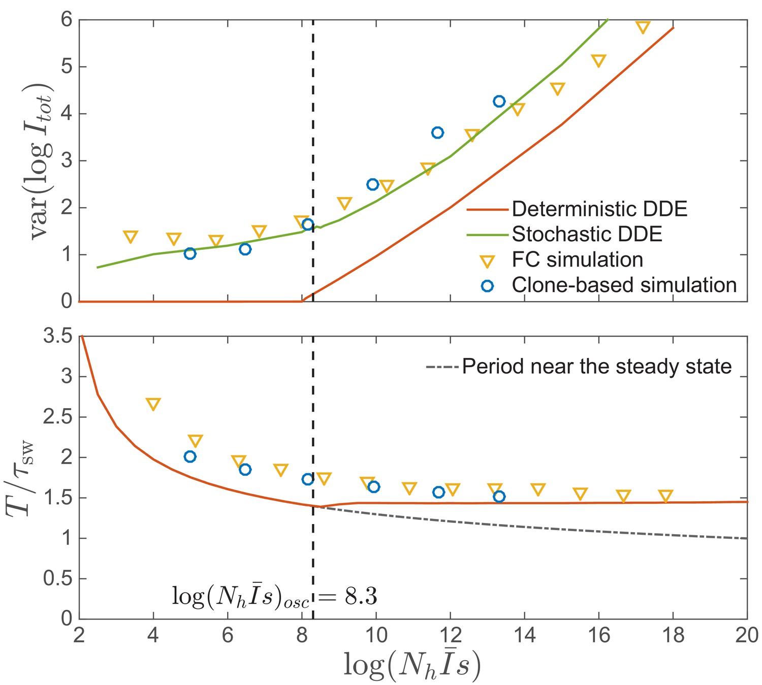
Amplitude and time scale of oscillations.
Top: Amplitude of epidemic circulations in logarithm of total prevalence. The amplitude predicted in the fitness class-based (FC) simulation is consistent with the clone-based simulation, bounded from below by the amplitude in the deterministic differential-delay approximation (DDE), which sets on at the spontaneous oscillation threshold , indicated by the dashed line. When the noise is properly considered as in Equation (15), the amplitude can also be predicted from the stochastic differential-delay equations (DDE). Bottom: Period of epidemic oscillation, also bounded below by the limit cycle period of the deterministic DDE.
Figure 4—figure supplement 2
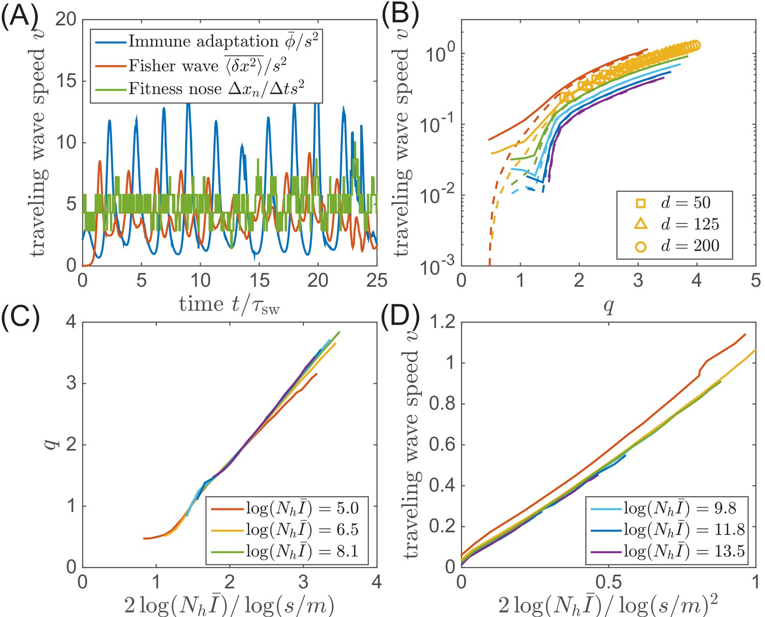
Speed of the traveling wave.
(A) In our model, the speed of traveling wave varies in time. The instantaneous speeds measured from immune adaptation, Fisher’s theorem, and nose advance could be different at any given moment. (B) But in the phase with steady traveling waves, the time-averaged speeds are consistent for different parameters. (C) The average nose position and (D) the average speed of adaptation (in the clone-based simulation) are consistent with the prediction of the traveling wave theory.
Figure 5
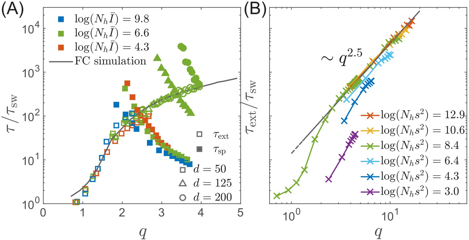
Extinction and speciation dynamics.
(A) Simulation results for the average extinction time (open symbols) and the average speciation time (filled symbols) as a function of pathogen diversity . The life time of the endemic RQS state is limited by the smaller of and . If , the population tends to speciate and persist, while the population is more likely to go extinct if . The graph shows and rescaled with the sweep time as a function of genetic diversity measured by the number of mutations . The speciation time increases with the range of cross-inhibition () and decreases with . Note the agreement between the results of the fitness class-based simulation (black line in (A)) and the clone-based simulation (colored squares in (A)). (B) Extinction time over a broad range of parameters, obtained via fitness class-based simulation of population dynamics, confirms its primary dependence on for large population sizes.
Figure 6
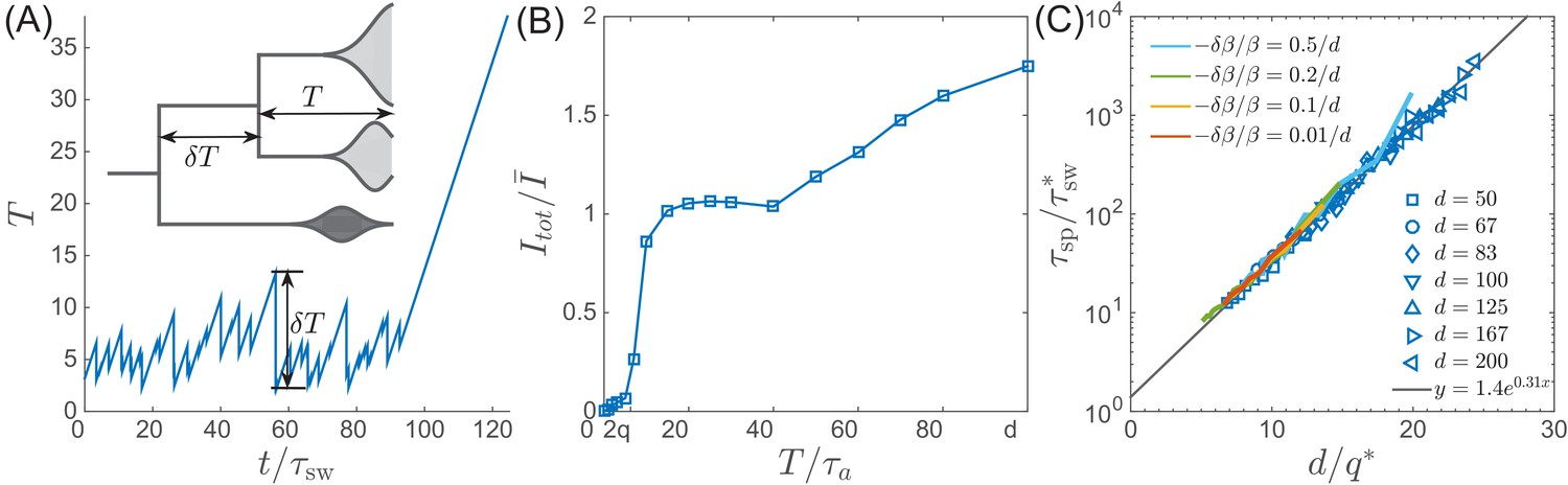
Speciation into antigenically distinct lineages.
(A) To speciate, two lineage have to diverge enough to substantially reduce cross-reactivity, that is needs to be comparable to . Inset: Illustration of the definition of time to most recent common ancestor and the time interval by which advances. (B) If such speciation happens, the host capacity - the average number of infected individuals increases two-fold. (C) The probability of such deep divergences decreases exponentially with the ratio , where effective antigenic diversity is . In the presence of deleterious mutations, the relevant is not necessarily the total advance of the pioneer strains, but only the antigenic contribution. This antigenic advance can be computed as with antigenic variance , where is fitness variance due to deleterious mutations. With this correction, speciation times agree with the predicted dependence (colored lines).
Figure 7
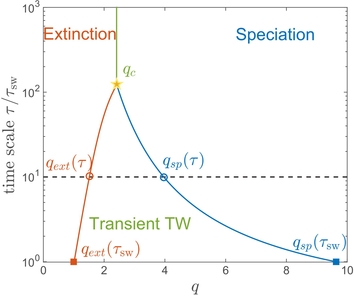
Lifetime of the RQS state.
This schematic diagram based on Figure 5A defines the ‘boundaries’ of the transient RQS (red line) and (blue line). gives the value of for which the average time to extinction is equal to is defined similarly but for the speciation process. Average times to speciation and extinction become equal at the critical value at which RQS persists the longest. For , and this value, along with the RQS lifetime, increases with .
Appendix 1—figure 1
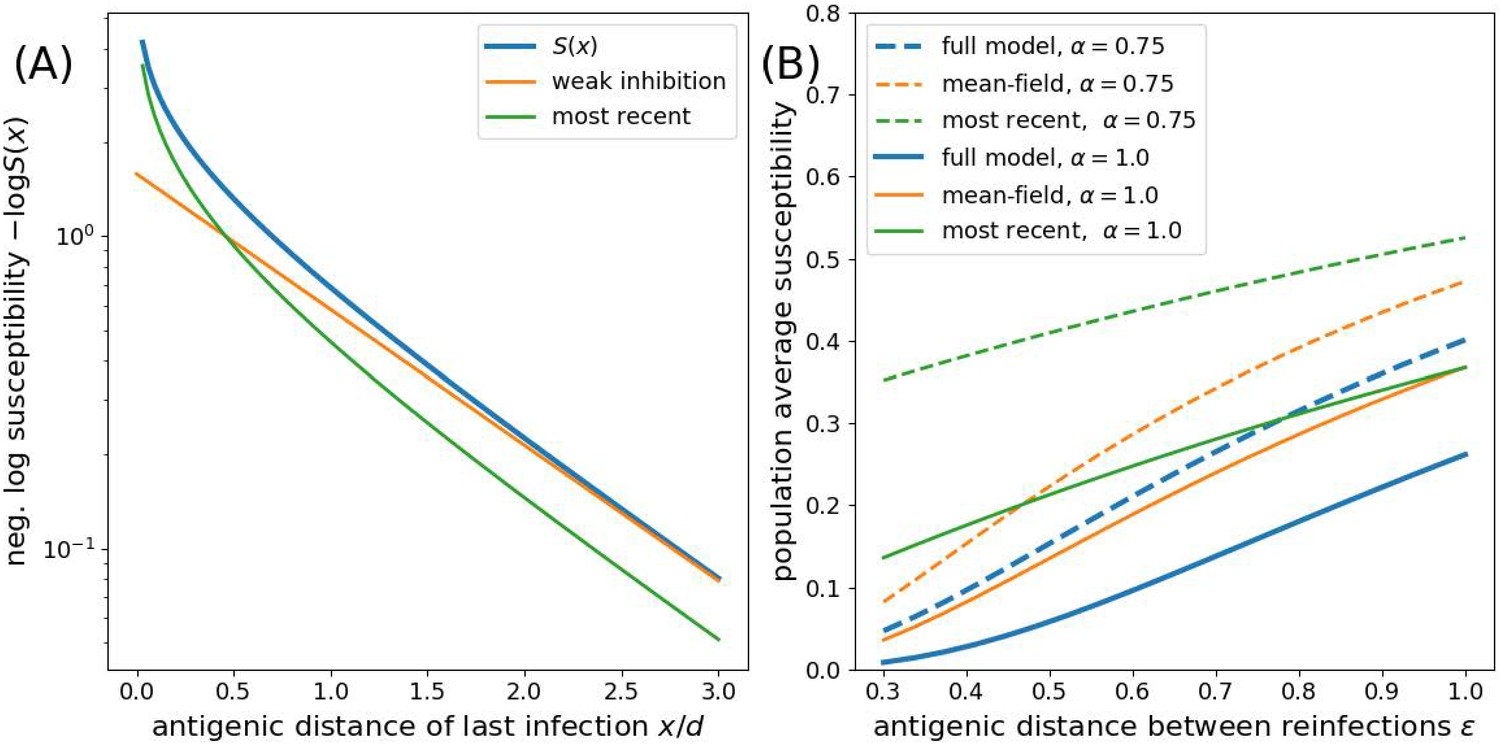
Approximations to the susceptibility.
Panel A shows the effect of approximating the multiplicative effect of all past infection by (weak inhibition) and by ignoring all by the most recent infection. Panel B shows the population average susceptibility assuming every individual gets reinfected once the virus has evolved by for the multiplicative model, the mean field approximation, and the most recent infection approximation for different values of as a function of the interval between infections .
Appendix 5—figure 1
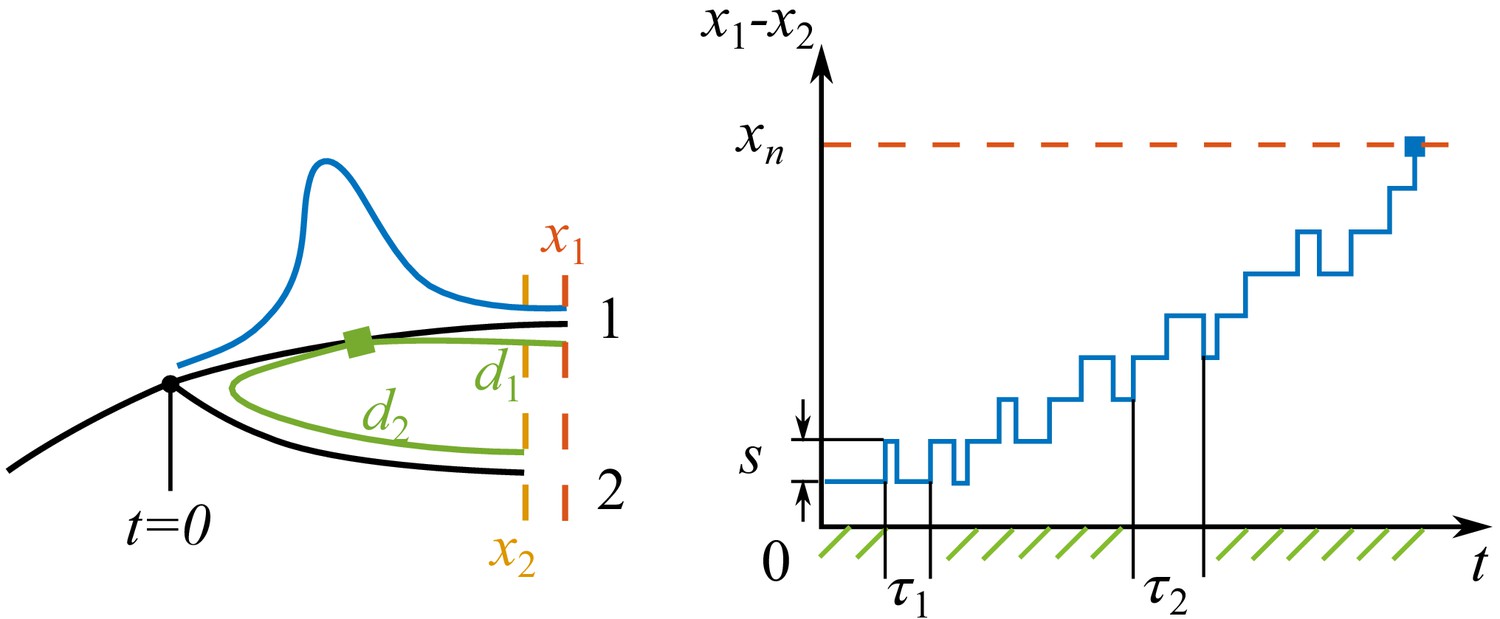
Process of speciation.
Left: Sketch of a branching event at with two branches 1 and 2. The fitnesses of the most fittest strains (noses) in branch 1 and 2 are and . Branch 1 is the fitter one . The antigenic distances from the cross-immune bulk to the noses of the two branches are and . The Gaussian profile in fitness is illustrated in blue. Right: The fitness difference between the two branches is doing a biased random walk in time of step size with a reflecting boundary at and an absorbing boundary at .
Tables
Table 1
Relevant quantities of influenza virus and parameters in multi-strain SIR model.
https://doi.org/10.7554/eLife.44205.013| Symbol | Definition | Typical values for influenza | Range in simulations |
|---|---|---|---|
| Fraction of population infected with strain | |||
| Population average susceptibility to strain | ∼0.5 | ||
| Total prevalence | |||
| Average total prevalence | 0.005 | ||
| Cross-immunity range | [50, 200] | ||
| Transmission rate | ∼0.5/day | 2 | |
| Recovery rate | ∼0.2/day | 1 (sets unit of time) | |
| Host birth/death rate | ∼0.01/year | 0 | |
| Cross-immunity of strains , | |||
| Coalescent time scale/sweep time | ∼2-6 years | ||
| Time to most recent common ancestor | ∼2-10 years | ||
| Fluctuations of | ∼2-6 years | ||
| Selection coefficient | ∼0.03/week | [0.003, 0.05] | |
| Beneficial mutation rate per genome | 10-3/week | [10-7,10-3] | |
| Host population | 1010 | [106, 1012] |
Additional files
-
Transparent reporting form
- https://doi.org/10.7554/eLife.44205.014
Download links
A two-part list of links to download the article, or parts of the article, in various formats.
Downloads (link to download the article as PDF)
Open citations (links to open the citations from this article in various online reference manager services)
Cite this article (links to download the citations from this article in formats compatible with various reference manager tools)
Phylodynamic theory of persistence, extinction and speciation of rapidly adapting pathogens
eLife 8:e44205.
https://doi.org/10.7554/eLife.44205


