Sub-second dynamics of theta-gamma coupling in hippocampal CA1
- Georgia Institute of Technology and Emory University, United States
- Georgia Institute of Technology, United States
Figures
Figure 1 with 6 supplements
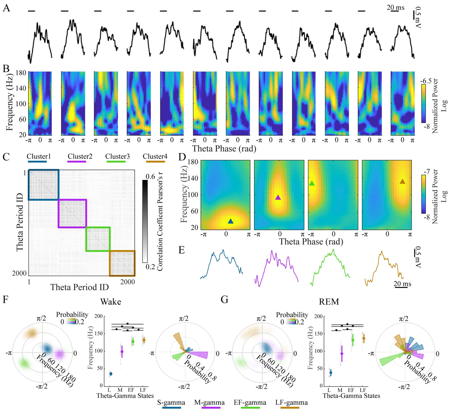
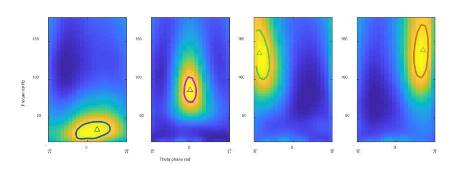
Clustering individual theta cycles based on cross-frequency coupling in hippocampal CA1.
(A) A raw LFP recording trace with twelve successive theta cycles from CA1 in an awake rat. (B) FPP for each theta cycle in A. (C) Correlation matrix of 2000 FPPs, organized based on k-means clustering. (D) Average FPPs across different theta cycles within the four clusters (n = 13720, 11404, 10745 and 14104 theta cycles from top to bottom) from one rat (Cicero, S09102014) during awake periods. Triangles indicate the center of gravity (see Materials and methods). (E) Individual example LFP traces for the four TG states, respectively. (F) Density plot of the frequency and theta phase for the center of gravity of the four types of gamma fields (fields were defined as 95% of peak value and above) detected from all rats during awake periods, left; frequency for the center of gravity (mean ± sd, n = 71 channels from 9 rats), middle, * denotes significant difference (paired t-test, q < 0.05, FDR correction for multiple comparisons); the distribution of theta phase for the center of gravity for the four TG states, right. (G) As in F from all rats during REM periods (mean ± sd, n = 64 channels from 8 rats). FPP: frequency and theta phase power. sd: standard deviation. TG: theta-gamma.
Figure 1—figure supplement 1
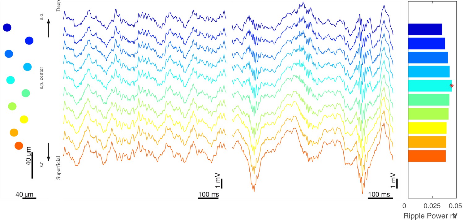
LFP recordings at different recording depths.
Example of recording sites on a Buzsaki probe (far left), traces showing theta oscillations (center left) and ripples (center right), and mean ripple power across channels with the channel with the maximum ripple power marked with a red star (far right). The channel with the maximum ripple power was used to identify the center of pyramidal layer in hippocampal CA1. Recording channels spanned 160–200 µm and most channels were in the pyramidal layer or immediately above or below it. s.o., stratum oriens; s.p. stratum pyramidal; s.r., stratum radiatum.
Figure 1—figure supplement 2
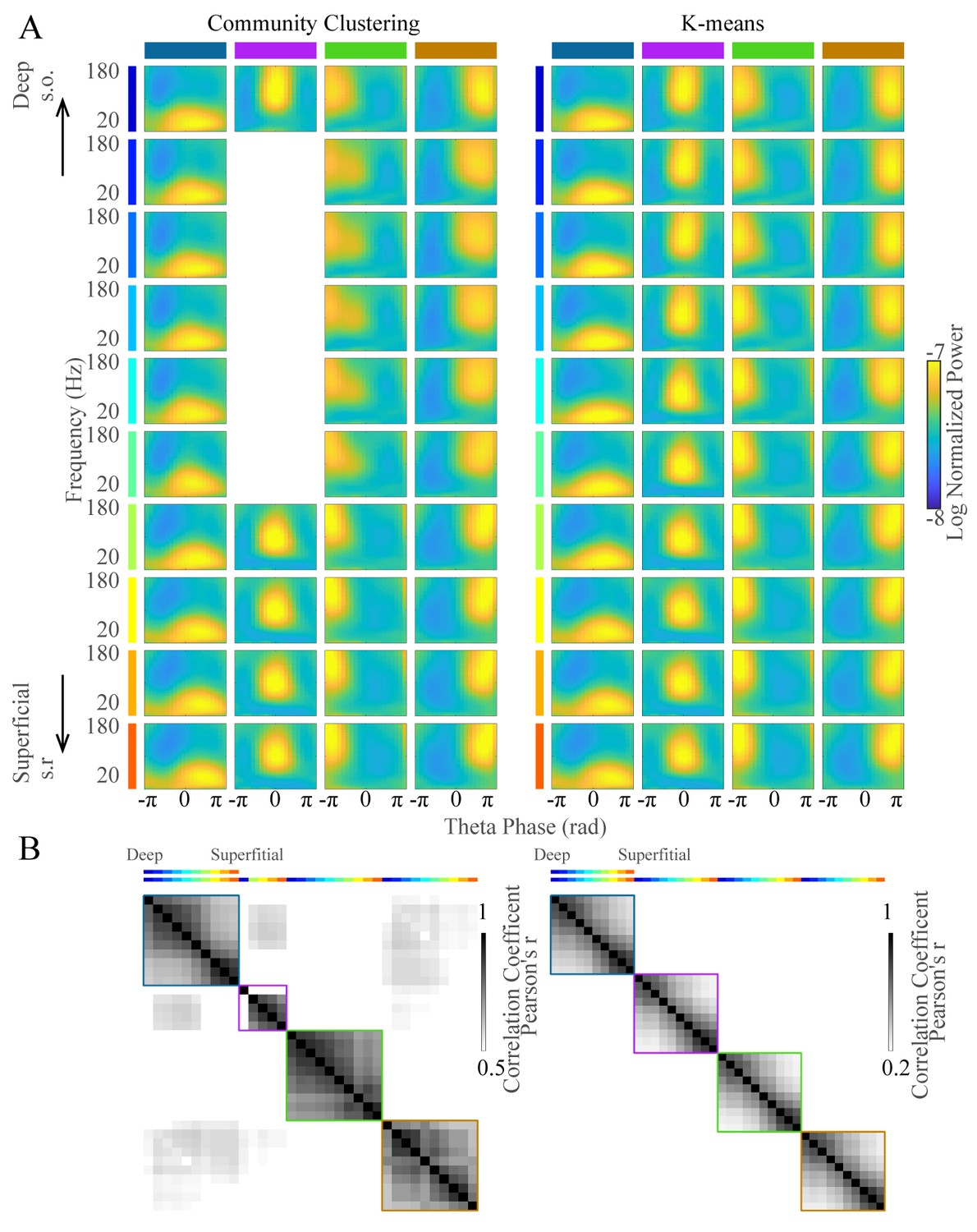
Clustering of wavelet power in frequency and theta phase domains.
(A) Average LFP power across frequency and phase for each cluster (columns) for all recording sites from deep to superficial channels (top to bottom) from the same shank of one probe. These data include all awake theta periods from one animal. (B) Correlation over time of the occurrence rate of each TG state between channels. The first row indicates the correlation overtime for theta cycles classified as in TG state one on the first channel correlated with the classification on all other channels. s.o., stratum oriens; s.r., stratum radiatum.
Figure 1—figure supplement 3

Averaged current source densities across channels for each TG cluster.
(A) Average FPP for each cluster for all recording sites from deep to superficial (top to bottom) from the same shank of one probe extracted from all awake periods from one animal (same as Figure 1—figure supplement 2, right). (B) Each cluster’s average current source density (CSD) as a function of frequency and theta phase. Clustering was performed on data from the channel identified as the center of the pyramidal layer (red rectangle in A). Current source densities were calculated over each three adjacent channels (dashed lines) and are shown from from deep to superficial channels (top to bottom). s.o., stratum oriens; s.r., stratum radiatum.
Figure 1—figure supplement 4

Intra-cluster sample correlation versus inter-cluster sample correlation.
Example distributions of the difference between intra- and the maximum inter-cluster correlation in two different animals.
Figure 1—figure supplement 5

Cross-validation for individual theta cycle assignments.
The top row represents the distribution of cross-validation accuracy of all data including inter-animal cross-validation (red), intra-animal cross-validation (black/gray), and intra-animal cross validation with a single fixed reference theta channel (fixed theta, light blue). The second (FPP calculated with local theta on the same channel) and third rows (FPP calculated with a fixed theta channel) show the intra-animal cross-validation separated for samples in each TG state (S-gamma, dark blue, M-gamma, purple, EF-gamma, green, LF-gamma, orange). The fourth row shows the inter-animal cross-validation separated for samples in each TG state. Solid line: mean; dash line: chance level.
Figure 1—figure supplement 6
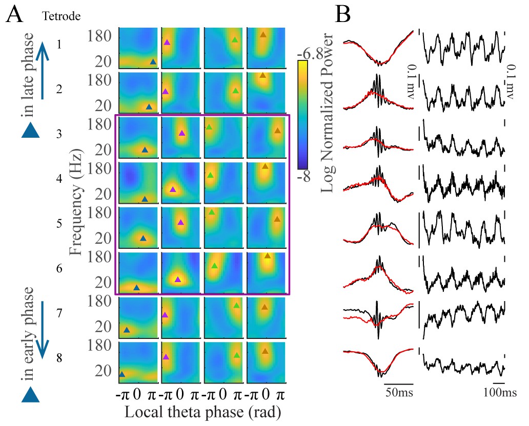
Clustering of tetrode data.
(A) Average FPP for each cluster (columns) for eight example tetrodes in CA1 during awake periods. Tetrodes are ordered by the gravity phase of S-gamma (late in the theta cycle, top, to early in the theta cycle, bottom). The purple rectangle indicates tetrodes with S-gamma at the peak of theta, similar to what was found using probe recordings from the channel with the largest ripple power. (B) Left: average LFP traces aligned to either the negative ripple peak (black) or ripple power (red, root mean square) during sleep, for each tetrode show in A. Right: Example LFP traces during theta periods for each tetrode shown in A.
Figure 2 with 4 supplements
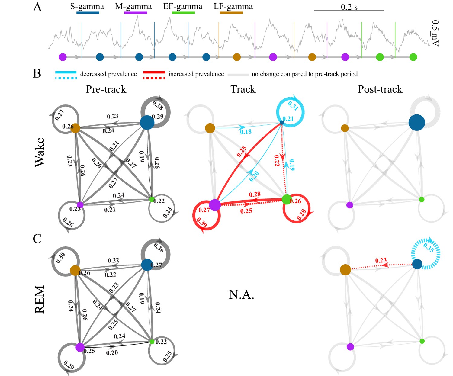
TG state transitions in awake and REM periods.
(A) An example LFP trace is shown with each theta trough marked by vertical lines and an illustration of TG state transitions below. (B) Transition matrices and occurrence probabilities of the four states summarized during pre-maze (left), maze (middle) and post-maze (right) periods respectively for all rats during awake periods (n=8 sessions from 4 animals in Hc-11). Paired t-tests were performed across pre-, post-, and maze periods for 20 dynamic parameters including 16 (4 states × 4 states) transitions and 4 state occurrences. Only significant changes from the pre-maze period (paired t-test, q < 0.05, FDR correction for 60 comparisons) are highlighted and color coded in red (increased prevalence) and blue (decreased prevalence), less strict statistics are highlighted by a dashed line for q < 0.1. (C) The same as B for REM periods. Because there is no REM during maze exploration, pre and post maze comparisons were made. None of the 20 parameters reached significance (paired t-test, q > 0.05, FDR correction for 20 comparisons); S-gamma→S-gamma and S-gamma→LF-gamma are reduced and enhanced respectively by using less strict statistics (q < 0.1, FDR correction for 20 comparisons).
Figure 2—figure supplement 1
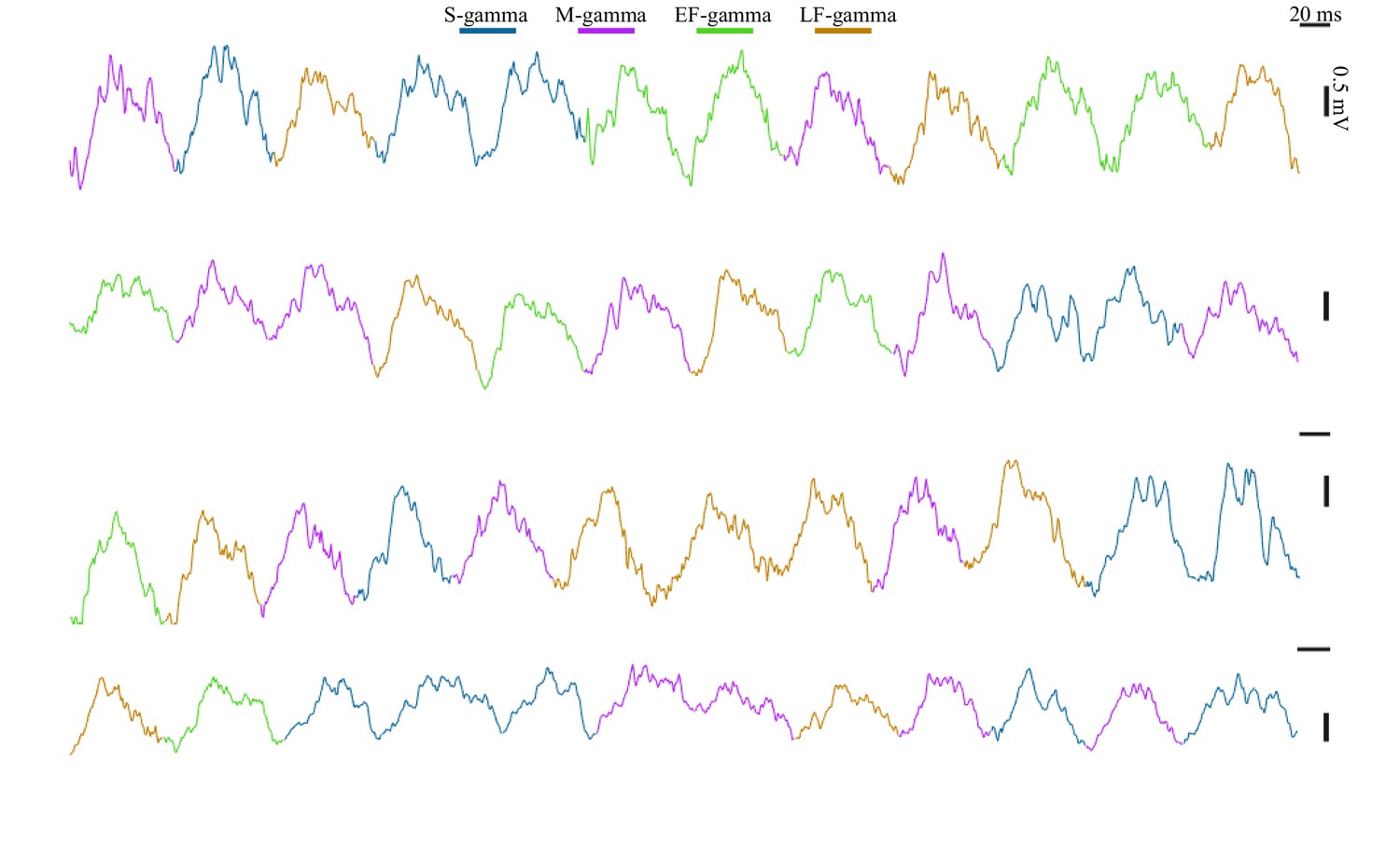
LFP examples during awake sessions.
LFPs recorded from four rats (each row is from one rat). Color codes denote clustering of individual theta cycles through k-means clustering.
Figure 2—figure supplement 2
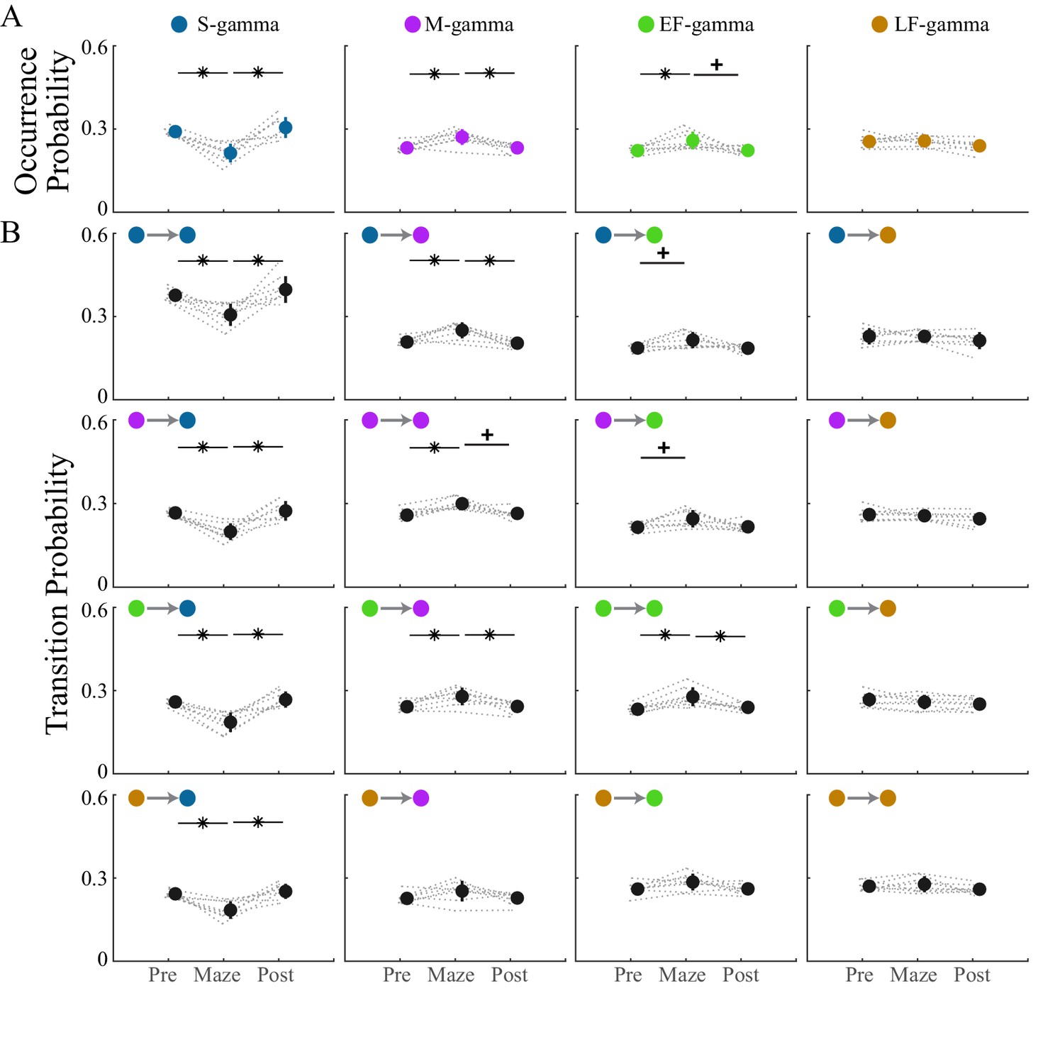
Transition matrix and occurrence of the four TG states during awake periods.
(A) TG state occurrence of the four states are presented in four graphs; comparisons are made across sessions. Note that in total 60 = [4 × 4 (transition matrix) + 4 (occurrence)] × 3 (pairs of session) comparisons are made (paired t test). (B) A 4 × 4 graph display shows the transition probability from the current state (row) to the next state (column); in each individual graph, the transition probabilities are compared across three experimental sessions (pre-maze period, maze period, and post-maze period). * denotes significant difference, FDR correction for 60 comparisons (q < 0.05); + denotes less strict statistics (q < 0.1).
Figure 2—figure supplement 3
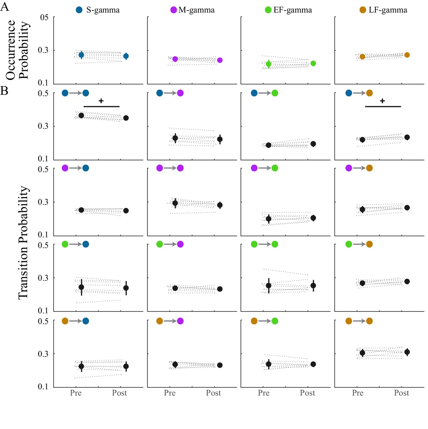
Transition matrix and occurrence of the four TG states during REM.
(A) TG state occurrence of the four states are presented in four graphs; comparisons are made across sessions. Note that in total 20 = [4 × 4 (transition matrix) + 4 (occurrence)] × 1 (pairs of session) comparisons are made (paired t test). (B) A 4 × 4 graph display shows the transition probability from the current state (row) to the next state (column); in each individual graph, the transition probabilities are compared across two experimental sessions (pre-maze period and post-maze period). + denotes significant difference, FDR correction for 20 comparisons (q < 0.1).
Figure 2—figure supplement 4
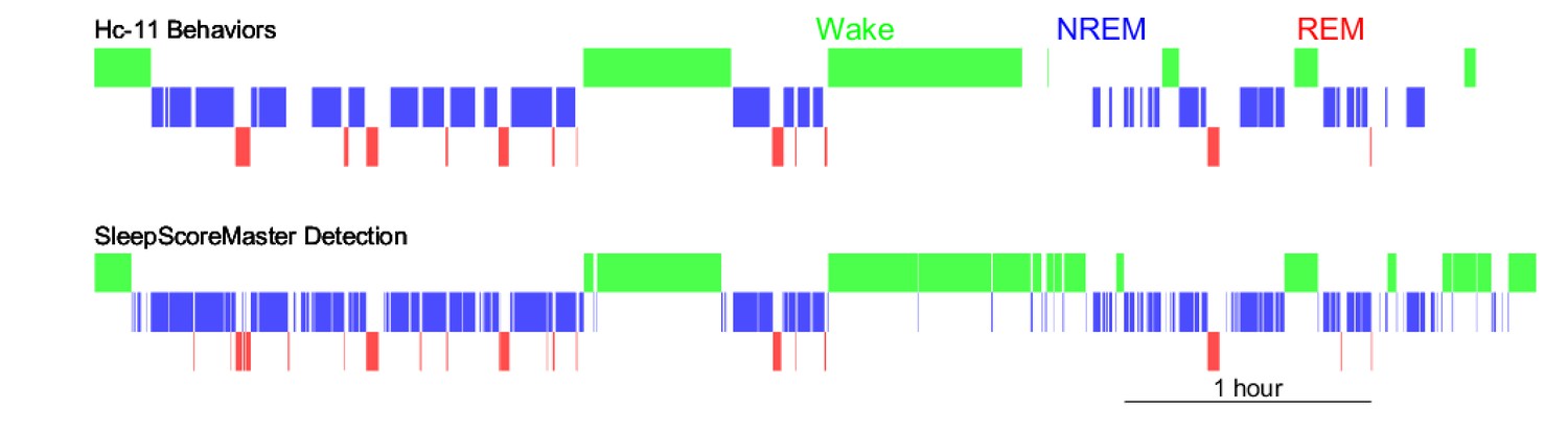
Automatic behavior state detection.
Wake (green), NREM (blue), and REM (red) periods detected by SleepScorreMaster (bottom) based on LFPs and LFP-reconstructed-EMG were similar to those detected manually (top) based on LFPs (theta-delta ratio), EMG, and video in one example rat.
Figure 3
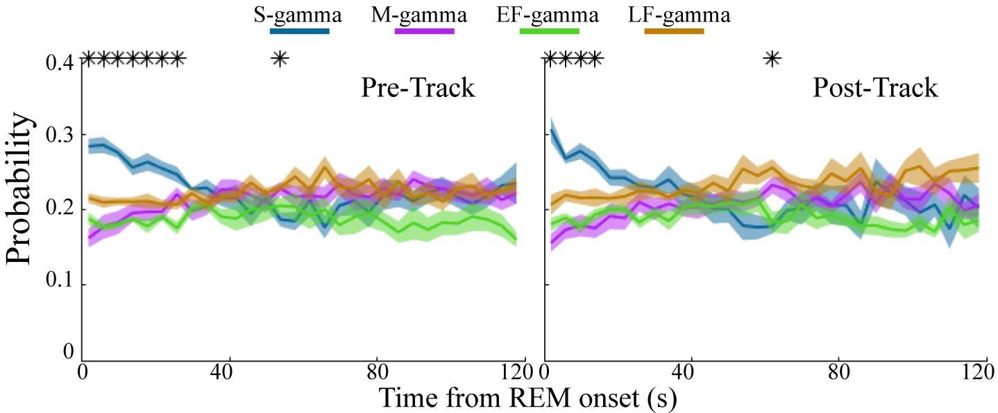
Low gamma dominates early REM.
State occurrence rates were calculated in 4s bins starting from REM onset from 0 to 120s for pre- and post-maze periods respectively (mean ± sem, n=8 sessions from 4 animals in Hc-11). * represents significant differences found across the four TG states (one way repeated measures ANOVA, q < 0.05, FDR correction for 30 comparisons). sem, standard error of the mean.
Figure 4
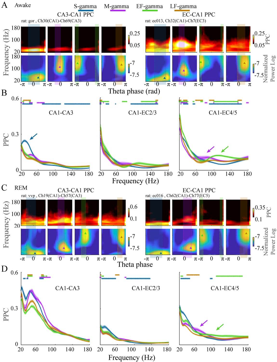
EC-CA1 and CA3-CA1 phase synchrony in the four TG states during awake and REM periods.
(A) Examples of CA3-CA1 pairwise phase consistency (PPC, top left) and EC-CA1 PPC (top right) as a function of frequency and theta phase for each TG state during awake periods. The corresponding CA1 spectrum is shown below and the highlighted region (translucent rectangle) was used to calculate the average PPC between LFPs (see Materials and methods). (B) Average PPC (mean ± sem, n=72 CA1-CA3 channel pairs from five sessions in two animals, n=17 CA1-EC2/3 channel pairs from five sessions in three animals, n=27 CA1-EC4/5 channel pairs from five sessions in three animals) within the highlighted theta phase interval in A across animals during awake periods. PPC was compared across TG states across frequencies (81 frequency samples from 20 to 180 Hz), TG states that were significant from all other states were highlighted by the corresponding color bar above (paired t-test, q < 0.05, FDR correction of 486 = 6 states pairs × 81 Frequency sample comparisons). (C) As in (A) but during REM periods. (D) As in (B) but during REM periods (n=8 CA1-CA3 channel pairs from one session in one animal, n=34 CA1-EC2/3 channel pairs from four sessions in three animals, n=22 CA1-EC4/5 channel pairs from four sessions in three animals). FDR: false discover rate. sem: standard error of the mean.
Figure 5 with 4 supplements
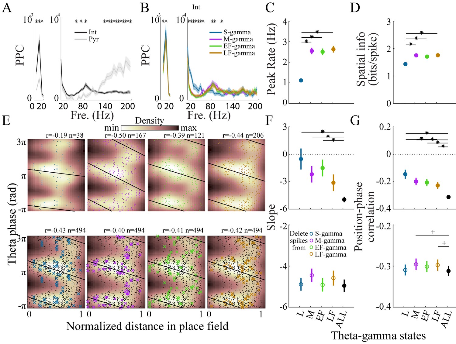
Interneurons and place cell activity in the four TG states.
(A) Spike-field pairwise phase consistency (PPC) for interneurons (n=100) and pyramidal cells (mean ± sem, n=266), * represents significant cell-type differences (one-way repeated measures ANOVA, q < 0.05, FDR correction from 33 comparisons). (B) Spike-field PPC of interneurons in the four TG states. * indicates significant differences across TG states (one way repeated measures ANOVA, q < 0.05, FDR correction from 33 comparisons). (C) Peak firing rate of place cells (n=142) for different TG states. * indicates significant differences (paired t test, q < 0.05, FDR correction for six comparisons). (D) Spatial information of place cells (n=142) for different TG states. * indicates significant differences (paired t test, q < 0.05, FDR correction for 6 comparisons). (E) Phase precession of an example unit (Unit 1008, rat Achilles S11012013) for four different TG states, thick black line shows phase-position regression (top). Phase precession of the same unit after randomly deleting 38 spikes (represented by ×), the minimum number of spikes of the four states, from each TG state (bottom). The place field entry and exit were normalized to 0 and 1, respectively, on the x axis; the phase-position correlation coefficient, r, is shown above each figure. (F) Slope of phase-position regression (n=142 fields) for each TG state (top panel) and after deleting spikes for each TG state (for each unit, results are averaged from 100 random deletions). Black dots indicate measures from including all spikes. * indicates significant differences (paired t test, q < 0.05, FDR correction for 10 comparisons); + indicates comparison reached significance threshold of q < 0.1. (G) As in (F) for phase-position correlation of the 142 place fields. sem, standard error of the mean.
Figure 5—figure supplement 1
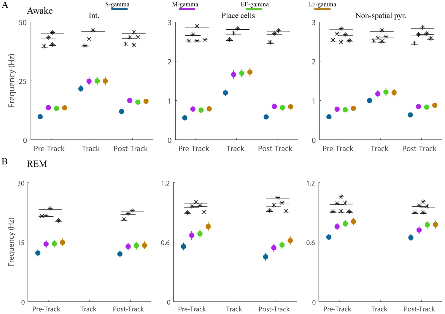
Firing rates of single units during the four TG states in awake periods.
(A) Firing rate of interneurons (left panel, n = 128), place cells (middle panel, n = 142), and non-spatial pyramidal cells (right panel, n = 420) are shown. * denotes significant differences, paired t test, FDR correction for the 18 = 6 (states pairs) × 3 (experiment sessions) comparisons (q = 0.05). (B) As in (A) but during REM periods. * denotes significant difference, paired t test, FDR correction for the 12 = 6 (states pairs) × 2 (experiment sessions) comparisons (q = 0.05). Circles indicate mean, error bars indicate standard error of the mean.
Figure 5—figure supplement 2
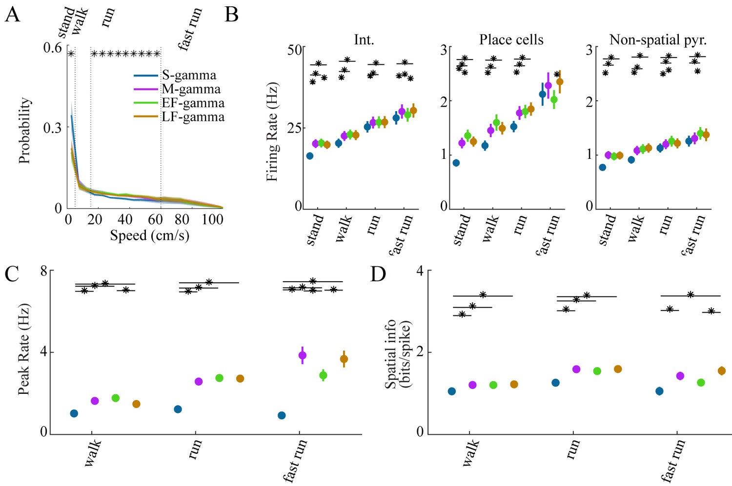
Neural firing properties across different animal speeds.
(A) Speed distribution from all animals in Hc-11 data sets for the four TG states (mean ± sem). * denotes significant differences, one-way repeated measures ANOVA, q < 0.05, FDR correction from 20 comparisons. 5, 15, 60 cm/s speeds represented by dashed lines separated four behaviors: stand, walk, run, and fast run. (B) Firing rates of interneurons, place cells, and non-spatial pyramidal cells during the four behaviors for four theta-gamma states, respectively. * denotes significant differences, paired t test, FDR correction for the 24 = 6 (states pairs) × 4 (behaviors) comparisons (q < 0.05). (C) Peak firing rate and (D) Spatial information of place cells during different TG states and behaviors. * denotes significant differences, paired t test, FDR correction for the 18 = 6 (states pairs) × 3 (non-standing behaviors) comparisons (q < 0.05). Circles indicate mean, error bars indicate standard error of the mean. sem, standard error of the mean.
Figure 5—figure supplement 3
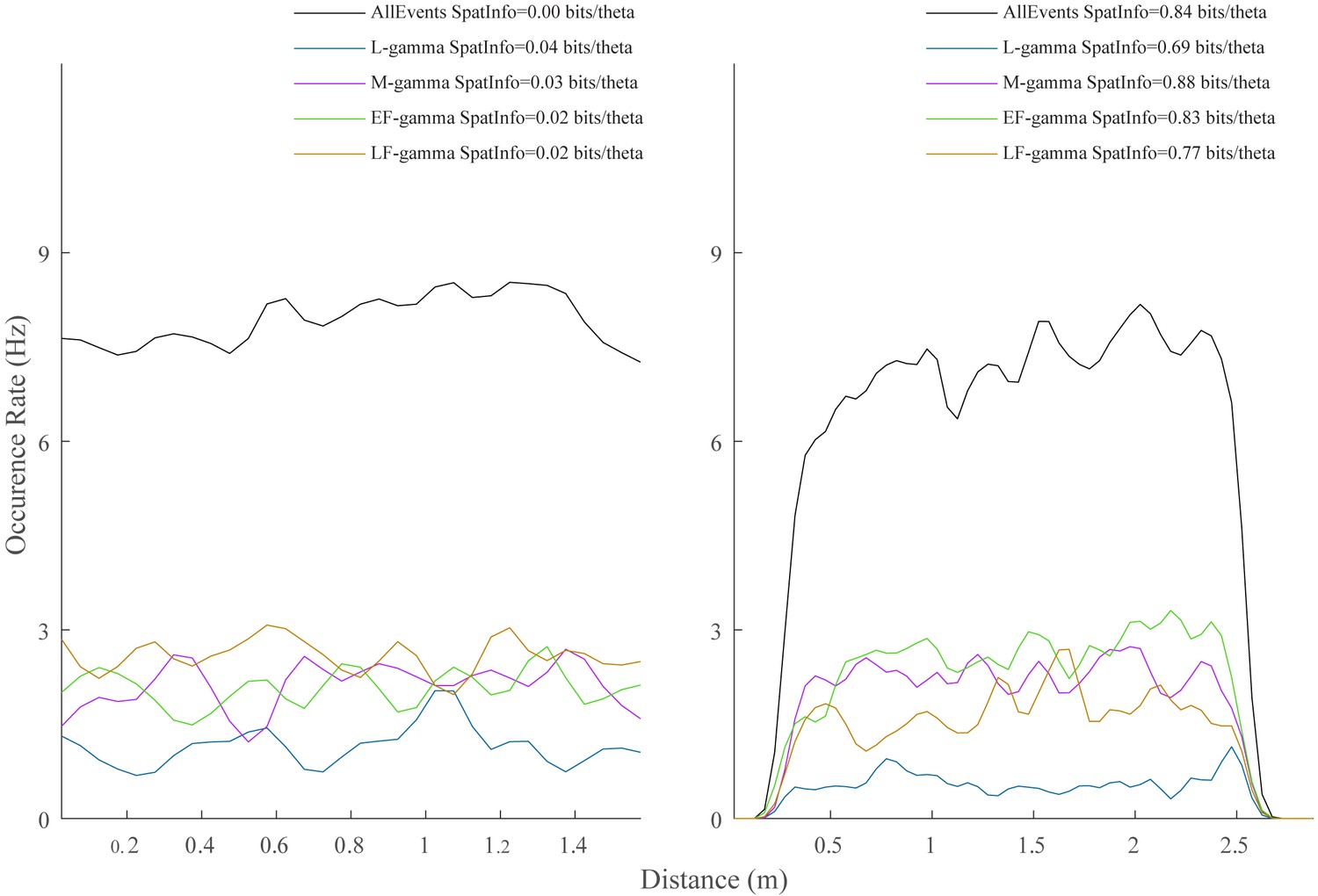
TG event occurrence as a function of animal spatial position.
Spatial occurrence rates of the four TG states for two example animals. Spatial information per TG state was also calculated, ranging from 0.01 to 0.90 bits/theta cycle for all animals in Hc-11 data sets.
Figure 5—figure supplement 4
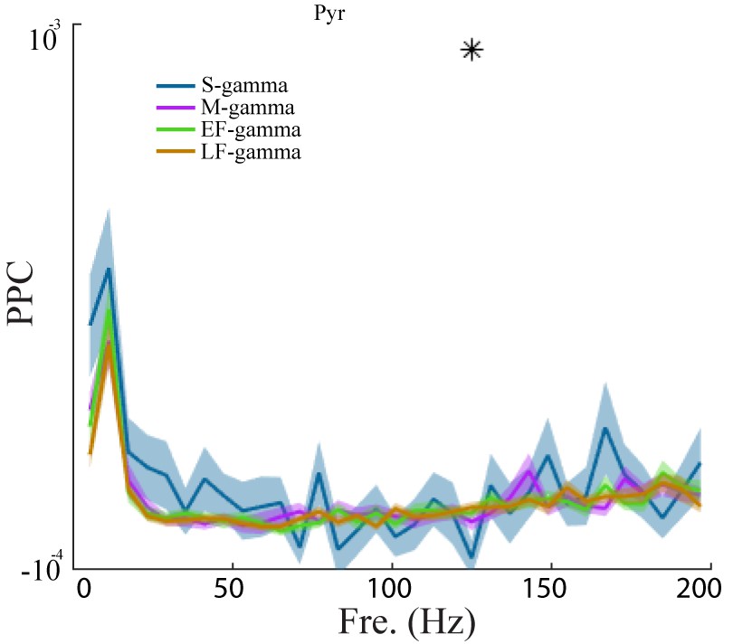
Pairwise phase consistency of pyramidal cells in the four gamma states.
PPC as a function of frequency for the four TG states (mean ± sem, n = 266 cells). * represents significant differences across gamma states (one way repeated measures ANOVA, q < 0.05, FDR correction from 33 comparisons). sem, standard error of the mean.
Author response image 1
FPS from 4 clusters identified using our shared code Solid line: gamma field defined as above 95% of the FPS peak value; triangles: gravity center.
Author response image 2

Theta Power across TG states.
The wavelet spectrum shown (2-20 Hz) was calculated for LFPs from Hc-11 data sets (n=48 channels) during awake pre-maze (left), maze (middle), and post-maze periods (right) over 2-200 Hz. The raw LFP power was normalized by dividing by the total power between 2 Hz and 200 Hz. Colored dots above indicate a TG state was significantly different from all other states (paired t-test, q < 0.05, FDR correction of 186 = 6 states pairs × 31 Frequency sample comparisons).
Tables
Table 1
Frequency and phase of gamma power fields for each TG state.
Frequency (mean ± sd) and phase (circular mean ± circular sd) for the centers of gravity of the mean FPPs for LFPs recorded from all animals in data sets Hc-11 and Hc-3 during awake (71 recordings in nine animals) and REM (64 recordings in eight animals) periods. sd: standard deviation.
| Wake (n = 71 recordings) | REM (n = 64 recordings) | |||
|---|---|---|---|---|
| FPP cluster | Frequency (Hz) | Phase (rad) | Frequency (Hz) | Phase (rad) |
| S-gamma | 36.07 ± 5.38 | 0.58 ± 0.51 | 39.28 ± 9.69 | 0.74 ± 0.53 |
| M-gamma | 99.12 ± 17.15 | −0.04 ± 0.88 | 93.36 ± 23.16 | −0.01 ± 0.96 |
| EF-gamma | 127.72 ± 11.28 | −2.57 ± 0.83 | 131.97 ± 17.31 | −2.67 ± 1.19 |
| LF-gamma | 131.83 ± 8.80 | 2.12 ± 0.77 | 136.80 ± 13.04 | 1.68 ± 0.88 |
Additional files
-
Supplementary file 1
Animal information.
Summary of experimental animals involved in the analysis. Note that TG state clustering was performed on all animals from both Hc-11 and Hc-3 data sets. Hc-11 data were specifically used for clustering analysis as well as TG state occurrence and transitions, spike-field analysis and place cell analysis. Hc-3 data were specifically used for CA3-CA1 and EC-CA1 LFP pairwise phase consistency analysis.
- https://doi.org/10.7554/eLife.44320.022
-
Transparent reporting form
- https://doi.org/10.7554/eLife.44320.023
Download links
A two-part list of links to download the article, or parts of the article, in various formats.
Downloads (link to download the article as PDF)
Open citations (links to open the citations from this article in various online reference manager services)
Cite this article (links to download the citations from this article in formats compatible with various reference manager tools)
Sub-second dynamics of theta-gamma coupling in hippocampal CA1
eLife 8:e44320.
https://doi.org/10.7554/eLife.44320


