Dissociable laminar profiles of concurrent bottom-up and top-down modulation in the human visual cortex
- Radboud University Nijmegen, Netherlands
- University Duisburg-Essen, Germany
Figures
Figure 1

Task design.
Plaid stimuli were presented in a block design. During stimulus blocks, eight stimuli were presented at a rate of 0.5 Hz (1.75 s on, 0.25 s off). Subjects were required to respond to each stimulus (except for the first in each block), indicating whether the bars in the cued orientation were thicker or thinner compared to the previously presented stimulus. Attention was cued by the colored fixation dot: red = clockwise, green = counter clockwise. Stimulus blocks were preceded by an attention cue and followed by performance feedback and an inter-block interval. See Materials and methods for more information on the task and stimuli.
Figure 2 with 1 supplement
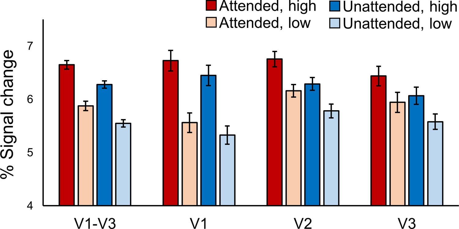
BOLD modulations from feature-based attention and stimulus contrast.
Average BOLD signal change in orientation-selective voxels from V1-V3 combined, and V1, V2 and V3 separately. In all areas responses to high contrast stimuli (darker bars) were higher than to low contrast stimuli (lighter bars). Responses were also higher in voxels that preferred the orientation that was attended (red bars) compared to those that preferred the ignored orientation (blue bars). Error bars show within-subjects standard error. See text for statistical details.
Figure 2—figure supplement 1
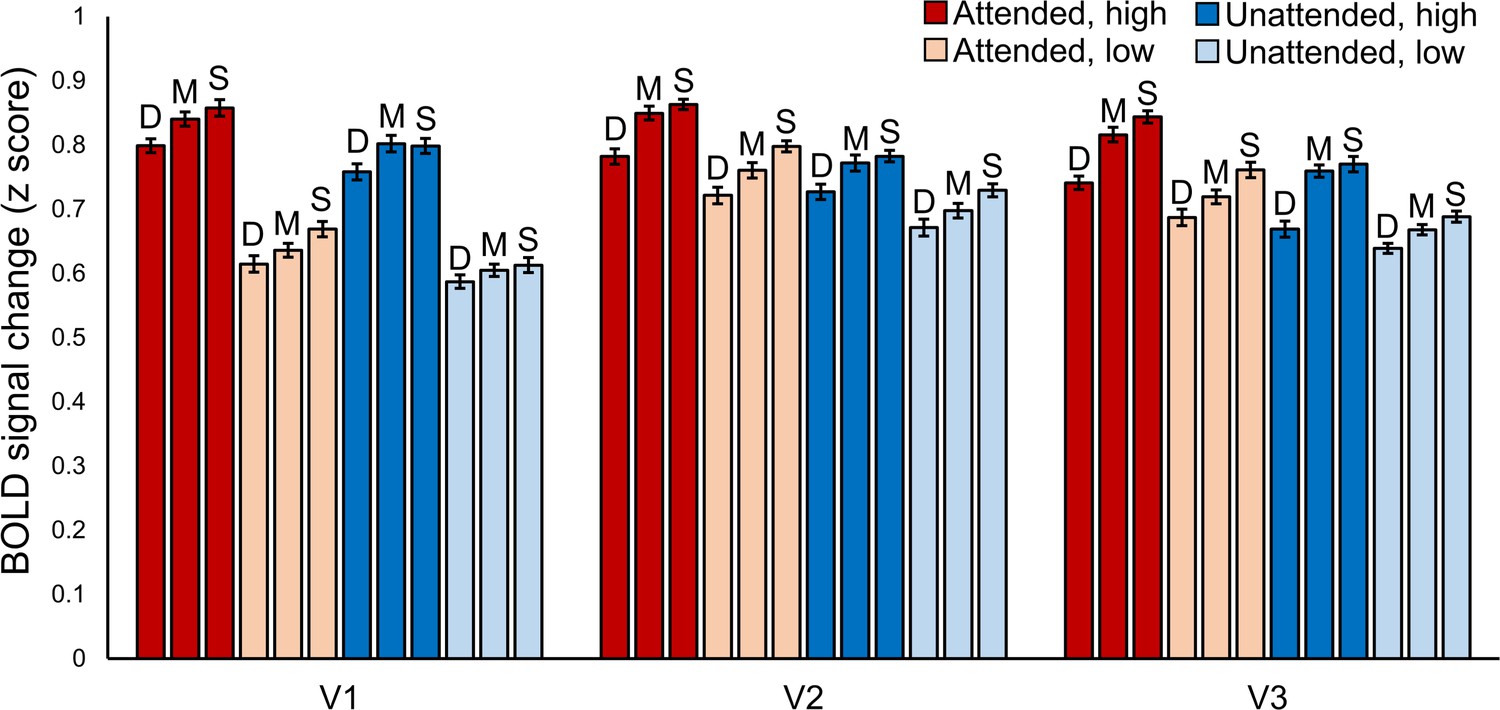
Layer-specific BOLD signal changes for each experimental condition.
Layer-specific BOLD signal change in orientation-selective voxels from V1, V2 and V3. In all areas responses to high contrast stimuli (darker bars) were higher than to low contrast stimuli (lighter bars). Responses were also higher in voxels that preferred the orientation that was attended (red bars) compared to those that preferred the ignored orientation (blue bars). For each condition signal change from deep, middle and superficial cortex is plotted from left to right (signified by D, M, S). Error bars show within-subjects standard error.
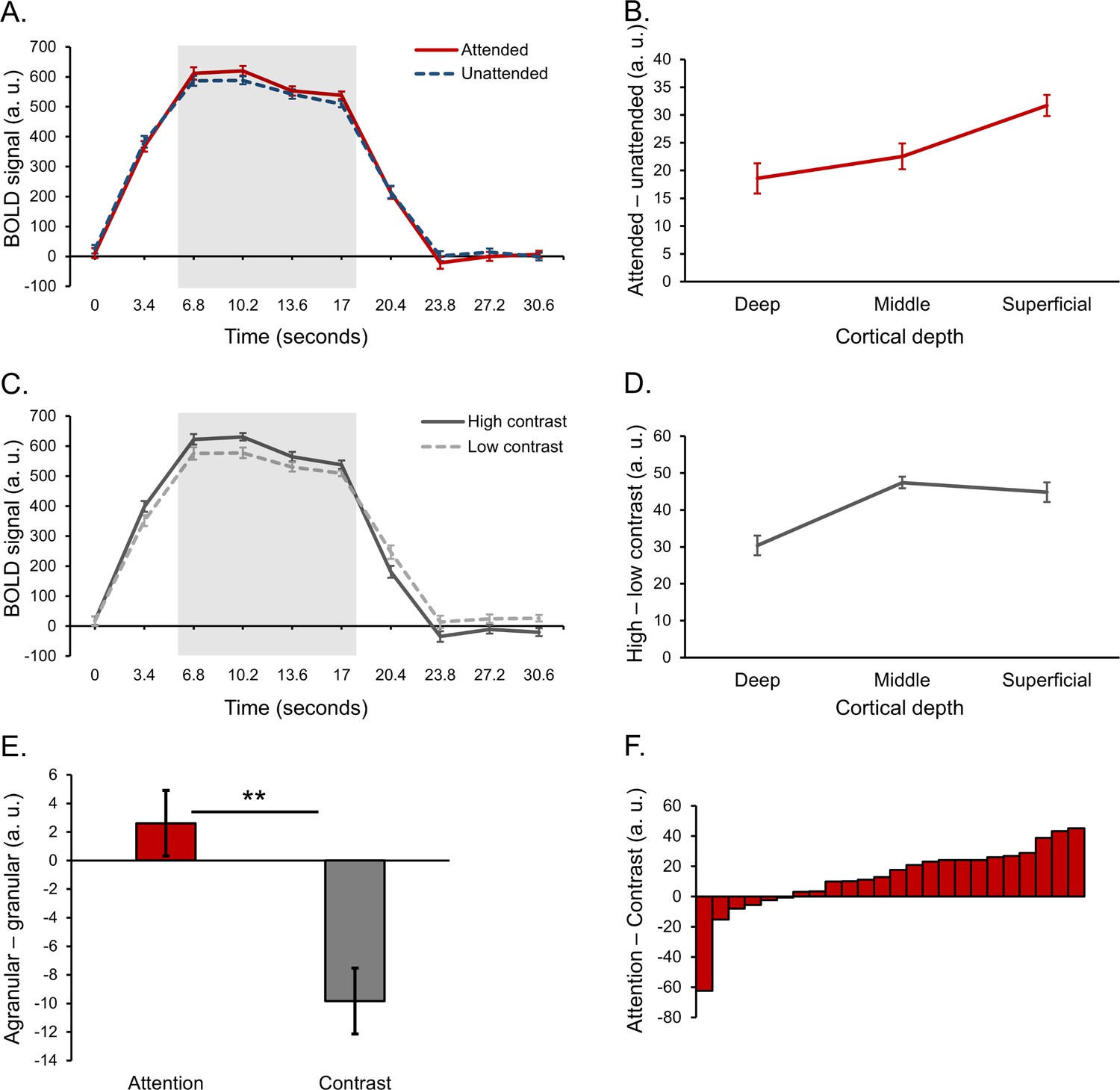
Figure 3 with 9 supplements

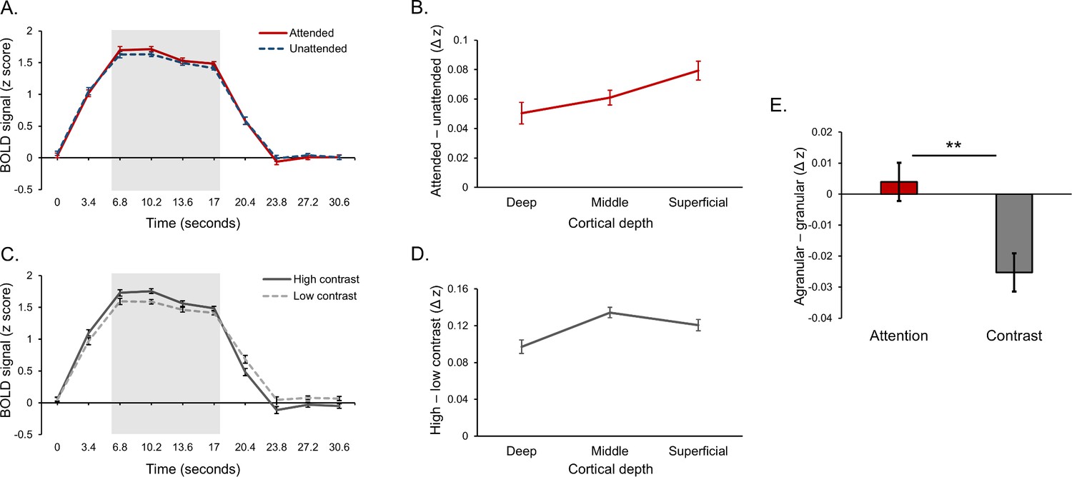
Laminar organization of top-down and bottom-up response modulations in V1-V3 combined.
(A) Average BOLD time course for a block of stimuli, averaged across cortical depth bins. Responses from voxels that preferred the attended orientation (red line) and voxels that preferred the unattended orientation (blue dash) are plotted separately. (B) Average difference between attended and unattended BOLD signals from the highlighted time points in panel A, plotted separately for cortical depth bins. (C) Average BOLD time courses for blocks of stimuli contained high (dark gray line) and low contrast (light gray dash) stimuli. (D) Average difference between responses to high and low contrast stimuli from the time points highlighted in panel C, plotted separately for cortical depth bins. (E) Group average scores indicating the whether the effects of attention (red bar) and contrast (gray bar) were stronger in the agranular or granular layers. Scores were computed by taking the average attention or contrast effect from the deep and superficial layers (left-most and right-most data point in panels B and D, respectively) and subtracting the attention or contrast effect from the middle layer (middle data point in panels B and D, respectively). A positive score indicates a more agranular response, negative indicates more granular. Asterisks denote a significant paired sample t test (p=0.005, see text for details). (F) Difference between agranular – granular scores (panel E) for attention and contrast conditions for each individual subject. A Positive score indicates that attention modulations were stronger in agranular layers compared to contrast modulations, which was the case for 20 out of 24 subjects. All error bars show within-subject standard error.
Figure 3—figure supplement 1
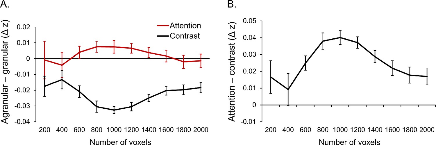
Effect of mask size on results.
In our main analysis, we constructed ROIs for V1, V2 and V3 comprising the 1000 most selective voxels (500 that preferred clockwise and 500 that preferred counter-clockwise). Here we conducted a series of control analyses to ensure our choice of 1000 voxels did not bias our results. (A) Agranular-granular scores for the effects of feature-based attention (red) and stimulus contrast (black) for a range of different mask sizes. (B) Difference between agranular-granular scores for the effects of attention and contrast plotted in panel A. A positive difference indicates that the effect of attention was more agranular compared to the effect of contrast. Though effect sizes varied with mask size, being smaller at the extremes (likely due to increased noise in laminar estimates when using few voxels and the inclusion of less selective voxels when using a large number of voxels), attention was more agranular than contrast for all mask sizes, as was the case in our main analysis. In both panels, error bars depict within-subject standard error.
Figure 3—figure supplement 2
Results using re-sampled orientation preference masks designed to sample from all cortical depths equally.
In our original analysis we selected voxels that were maximally responsive to and selective for our stimuli. This included restricting ROIs to only include voxels that exhibited a significant response to the stimuli presented in the stimulus localizer. Due to stronger overall signal in superficial cortex, this restriction created a sampling bias where our masks included more voxels that maximally overlapped with the superficial depth bin compared to other bins: on average in V1, 334 voxels (SD = 97) maximally overlapped with the superficial bin, compared to 141 (SD = 43) for middle and 175 (SD = 55) for deep. Similarly, for V2 there were 331 voxels (SD = 117) for superficial, 146 (SD = 50) for middle and 189 for deep (SD = 56) and in V3 there were 379 voxels (SD = 132) for superficial, 162 (SD = 55) for middle and 177 (SD = 54) for deep. Note that the total number of voxels reported here for each visual area do not add up to the total analyzed for each visual area (1000). This is because there were also a number of voxels that fell within white matter and CSF, which helped the spatial GLM estimate responses for these depth bins that fell outside the gray matter, but responses from these depths were not analyzed further. To check our results were not dependent on this sampling bias, we conducted the following control analysis. We resampled our orientation preference masks by randomly removing voxels until there was an equal number that maximally overlapped with each gray matter depth bin. This resulted in 132 voxels (SD = 40) for each depth bin in V1, 137 (SD = 46) for each depth in V2, and 141 (SD = 45) for each depth in V3. We recomputed our analyses using these control masks that sampled evenly from all cortical depths, which revealed very similar results. The effect of attention was significant during the highlighted time points (stats, panel A). The effect of attention varied across depth (F [46, 2]=3.55, p=0.037, panel B), being larger in superficial compared to middle (t [23]=2.05, p=0.052) and deep cortex (t [23]=2.25, p=0.034). The effect of stimulus contrast was significant in the highlighted time window (stats, panel C). The effect of contrast varied significantly across depth (F [46, 2]=5.73, p=0.006), being larger in the middle depth bin compared to deep (t [23]=3.20, p=0.004, panel D). The effect of attention was significantly stronger in the agranular layers compared to stimulus contrast (t [23]=2.37, p=0.026, panel E). Overall, the results of this control analysis were similar to our main analysis. All error bars depict within-subjects standard error.
Figure 3—figure supplement 3
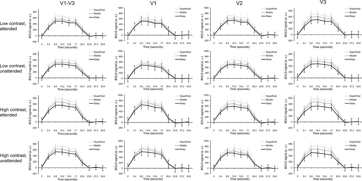
Raw layer-specific time courses for each condition and visual area.
Raw group average time courses are plotted for each condition (from top to bottom: low contrast attended, low contrast unattended, high contrast attended, high contrast unattended) and for each visual area (from left to right: V1-V3 combined, V1, V2, V3). Time courses from deep (black lines), middle (dark gray lines) and superficial (light gray lines) layers are plotted separately. These average time courses were computed using raw layer-specific time courses, before they were normalized using within-layer z scoring (described in Materials and methods), showing the bias in signal strength towards superficial cortex in the raw data. Error bars show within-subject standard error.
Figure 3—figure supplement 4
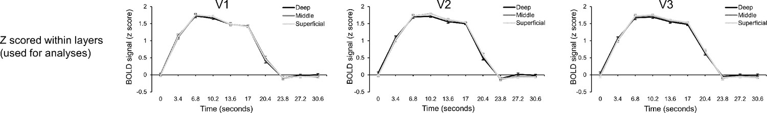
Removal of layer-specific BOLD bias.
As expected, there was a bias in overall BOLD amplitude towards superficial cortex (see Figure 3—figure supplement 3). For the analyses reported in our main paper, we removed this bias by z scoring data within layers, after we had estimated layer-specific responses from the pre-processed voxel data. The figure shows normalized layer-specific time courses from V1, V2 and V3, averaged across experimental conditions. The bias in BOLD amplitude in superficial cortex is almost completely removed.
Figure 3—figure supplement 5
Main results using raw layer-specific time courses with no normalization.
Our main results (shown in Figure 2) were obtained using layer-specific time courses that were normalized by z scoring data within layers. It was possible that normalizing in this manner could have impacted our effect sizes of interest. This is because the standard deviation across a time course, the denominator in a z score calculation, is somewhat dependent on the size of response fluctuations caused by our manipulations of attention and contrast. To determine whether this was the case, we repeated all the analyses from Figure 2 of raw layer-specific time courses without any normalization. The figure shows that both the attention (panel A) and contrast (panel C) effect sizes appear very similar to those in Figure 2, indicating that any effect of within-layer z scoring on effect sizes was negligible. Layer-specific effects (panel B, D–F) are also highly similar to those reported in our main analysis in Figure 2. All error bars depict within-subjects standard error.
Figure 3—figure supplement 6
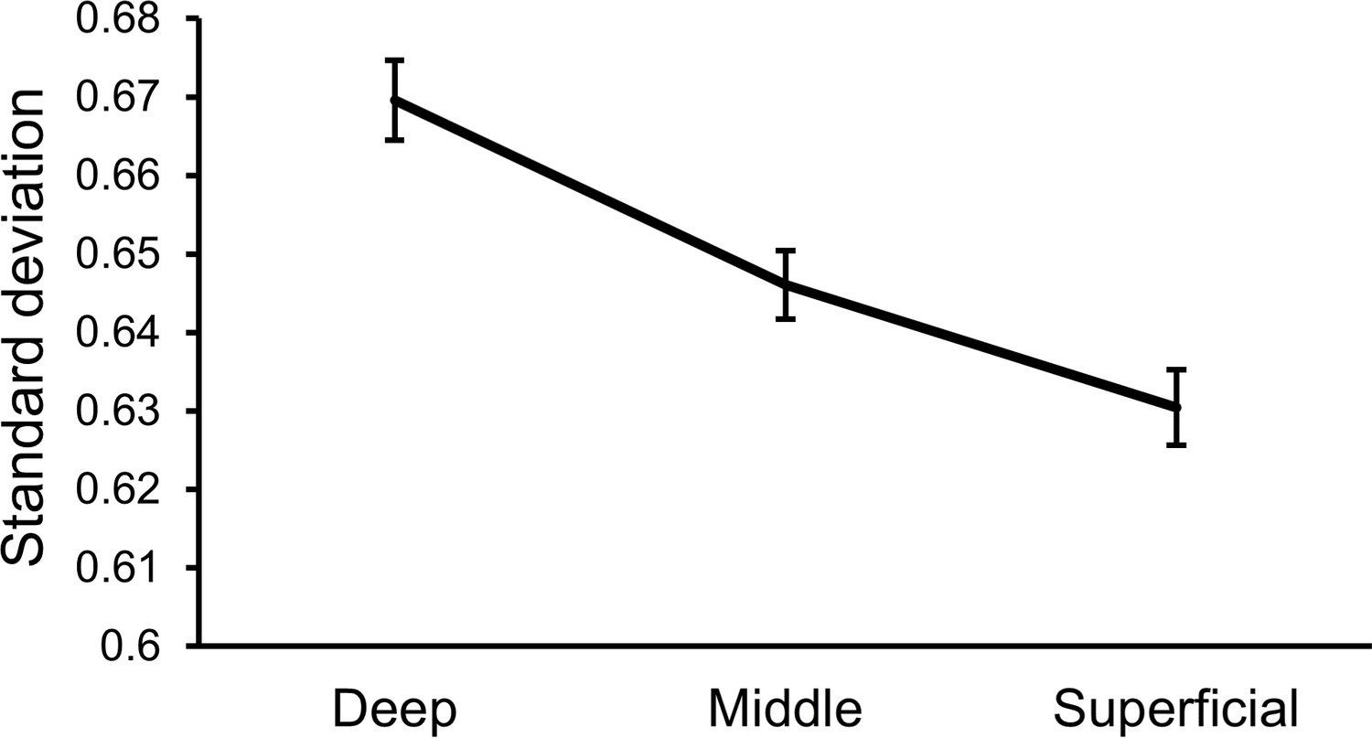
Differences in trial-to-trial variance between cortical layers.
To see if there were differences in signal variance between cortical layers, we computed trial-to-trial standard deviation in our (normalized) layer-specific time courses for each of the 10 time points within a single trial, and then computed the average standard deviation across time points. The group average standard deviation for each layer clearly shows a difference in overall signal variance between layers, where variance was higher in deeper cortex (F [46, 2]=11.41, p=9.5e-5). It therefore appears that signals we measured from deeper cortex had overall lower signal strength and larger variance. Error bars show within-subject standard error.
Figure 3—figure supplement 7
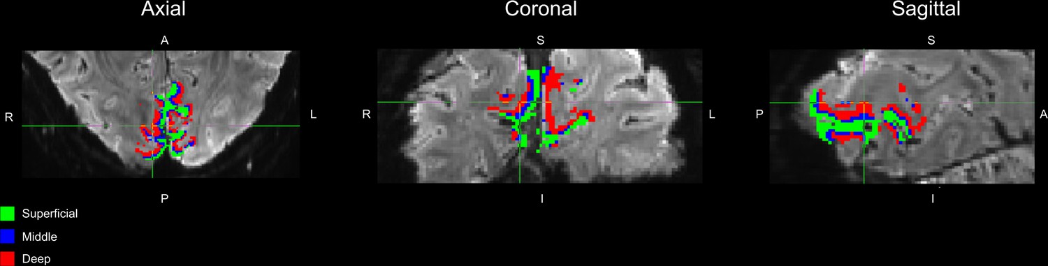
Example cross section of V1 mask.
Axial (left), coronal (middle) and sagittal (right) views of a cross section of one example subject’s V1 mask. Superficial, middle and deep voxels are colored in green, blue and red, respectively. Note that in our spatial GLM approach (described in Materials and methods), voxels’ contributions to layer-specific time courses were weighted by their proportion overlap with each layer. For the purposes of visualization in this figure, voxels are labeled according to which layer they maximally overlapped with.
Figure 3—figure supplement 8
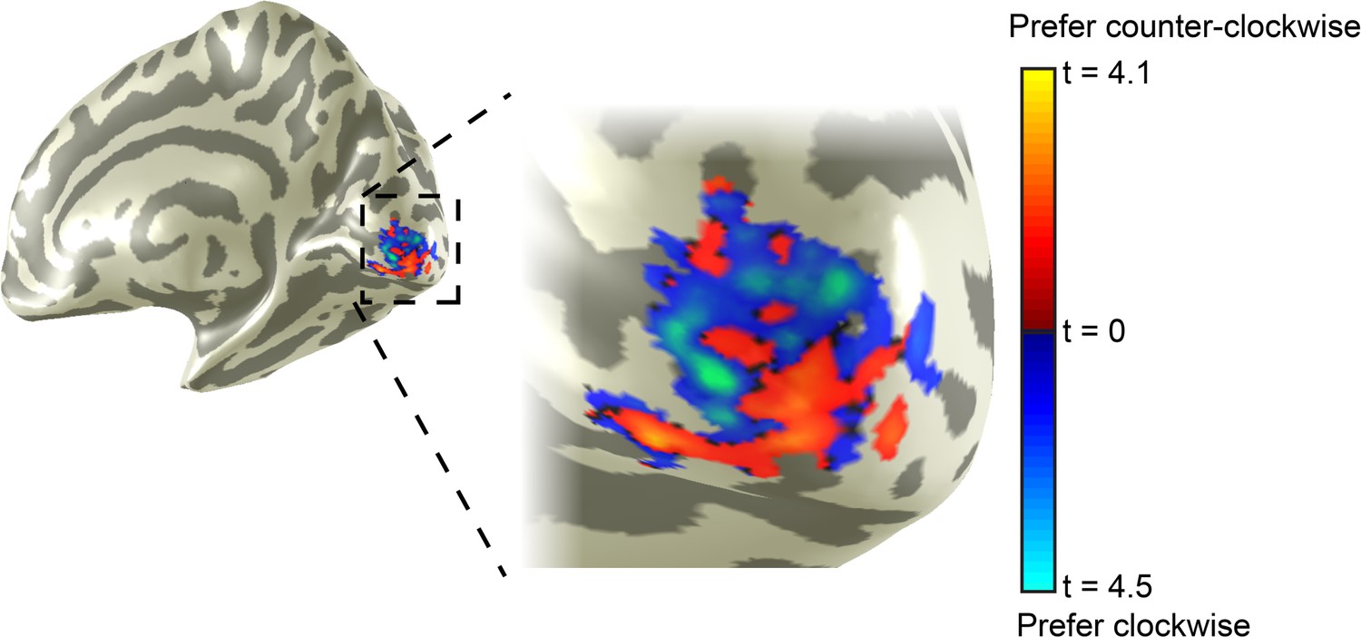
Layout of orientation-selective voxels in V1.
Example V1 clockwise (blue-light blue) and counter-clockwise (red-yellow) masks for one representative subject. Brighter colors indicate stronger selectivity for the preferred orientation (t statistic, see Materials and methods for more details).
Figure 3—figure supplement 9
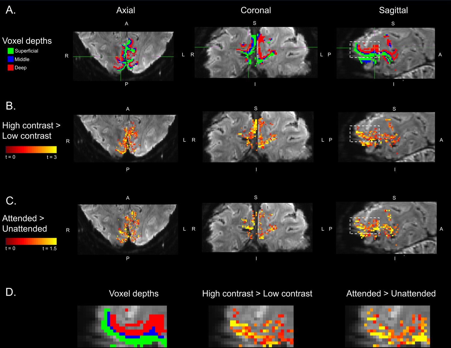
Example layer-specific masks and statistical maps.
(A) Axial (left), coronal (middle) and sagittal (right) views of a cross section of one example subject’s V1 mask. Superficial, middle and deep voxels are colored in green, blue and red, respectively. Note that in our spatial GLM approach (described in Materials and methods), voxels’ contributions to layer-specific time courses were weighted by their proportion overlap with each layer. For the purposes of visualization in this figure, voxels are labeled according to which layer they maximally overlapped with. (B) Statistical map showing voxel t values for the high contrast >low contrast stimuli from the main analysis for the same slices in panel A. (C) Statistical map showing voxel t values for attended >unattended orientation from the main analysis for the same slices in panel A. (D) Zoom in on a region of cortex highlighted by the white dashed boxes in sagittal views in panels A-C. By comparing voxels depths (left), contrast (middle) and attention (right) t maps, it can be seen that middle-depth voxels tend to show larger contrast modulation, while superficial voxels are more modulated by attention.
Figure 4

Laminar organization of top-down and bottom-up response modulations in V1, V2 and V3.
(A) Average difference between depth-specific time courses in voxels that preferred the attended orientation and voxels that preferred the unattended orientation in V1 (orange), V2 (blue) and V3 (green). (B) Average difference between depth-specific time courses from blocks containing high and low contrast stimuli for V1, V2 and V3. (C) Average difference between attention modulations (taken from panel A) and contrast modulations (from panel B) in the agranular layers (average of deep and superficial bins) and granular layer (middle bin) for V1, V2 and V3. A positive score indicates a more agranular response, negative indicates more granular. All error bars show within-subject standard error.
Author response image 1
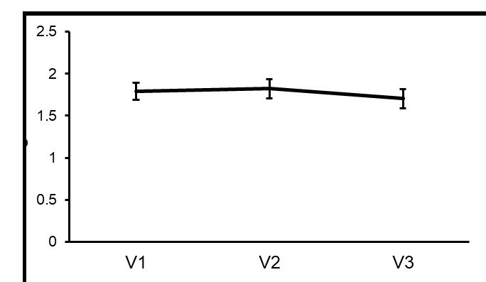
Differences in orientation selectivity across areas.
The average unsigned t value for the clockwise > counter-clockwise contrast that was applied to the orientation localizer data are plotted for all voxels within orientation-selective masks in V1, V2 and V3.
Additional files
-
Transparent reporting form
- https://doi.org/10.7554/eLife.44422.017
Download links
A two-part list of links to download the article, or parts of the article, in various formats.
Downloads (link to download the article as PDF)
Open citations (links to open the citations from this article in various online reference manager services)
Cite this article (links to download the citations from this article in formats compatible with various reference manager tools)
Dissociable laminar profiles of concurrent bottom-up and top-down modulation in the human visual cortex
eLife 8:e44422.
https://doi.org/10.7554/eLife.44422


