Dynamic control of hippocampal spatial coding resolution by local visual cues
Figures
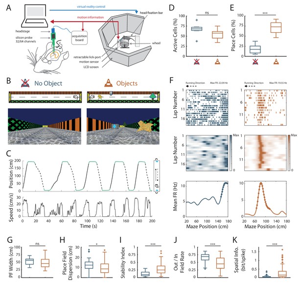
Effects of local visual cues on spatial coding resolution .
(A) Schema of the virtual reality set up. The mouse is head-fixed and located on a wheel surrounded by LCD screens where a virtual environment is displayed. (B) Top and first person views of virtual linear tracks used. Left: track without objects (ØT) and right: track with virtual 3D objects (OT). (C) Top: Animal’s position in the virtual track as a function of time. Green lines indicate times when animal was in a reward zone location. These locations were not considered for further analysis. Solid and dotted black lines indicate back and forth trials respectively. Top view of animal in the maze is depicted on the right. Arrows indicate teleportation in the same position but facing opposite direction after reward consumption. Bottom: Animal’s speed as a function of time. (D,E) Box plots of the percentage of active cells (D) and place cells (E) in the maze without (blue) and with (orange) objects (same color code throughout the figures). (F) Spike raster plots (top) and color-coded firing rate map (middle) for successive trials in one direction (arrow) as a function of the position in the maze. Bottom: corresponding mean firing rate by positions. Dots indicate positions of the detected place field (see Materials and methods). (G–K) Box plots of the place field width (G), the place field dispersion (H), the stability index (I), the out/in field firing rate (J) and the spatial information (K). For box plots in this and subsequent figures, box extends from the first (Q1) to the third quartile (Q3) with the band inside showing the median and the extremities of the whiskers include values greater than Q1-1.5*(Q3-Q1) and smaller than Q3 +1.5*(Q3-Q1).
-
Figure 1—source data 1
Source data for Figure 1.
- https://doi.org/10.7554/eLife.44487.005
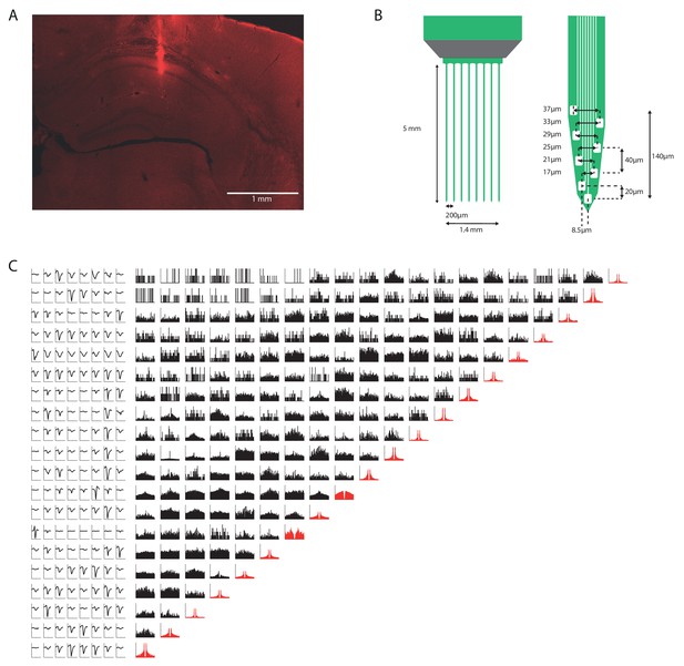
Histology and spike sorting.
(A) Representative histology slide showing a silicon probe track ending in CA1 pyramidal layer. Scale bar: 1 mm. (B) Probe details: Shank and recording channels spacing (C) (Right) Auto-correlograms (red) and cross-correlograms (black) of 20 CA1 units recorded simultaneously. (Left) Average units waveforms (for visualization each row is normalized by the unit maximum average waveform).

Effects of local visual cues on spatial coding resolution across different recording sessions.
(A–D) Box plots of the place field dispersion (A; ØT: 12.1 ± 0.65 cm, n = 8 recording sessions; OT: 9.69 ± 1.13 cm, n = 8 recording sessions; t14 = 1.86, p=0.08, two-tailed unpaired t-test), the stability index (B; ØT: 0.14 ± 0.02, n = 8 recording sessions; OT: 0.29 ± 0.04, n = 8 recording sessions; t14 = −3.39, p=0.0044, two-tailed unpaired t-test), the out/in field firing rate (C; ØT: 0.65 ± 0.03, n = 8 recording sessions; OT: 0.45 ± 0.04, n = 8 recording sessions; t14 = 4.40, p=0.0006, two-tailed unpaired t-test) and the spatial information (D; ØT: 0.06 ± 0.02, n = 8 recording sessions; OT: 0.27 ± 0.05, n = 8 recording sessions; Z = −2.88, p=0.0038, two-tailed unpaired t-test) without (blue) or with (orange) objects between different recording sessions.
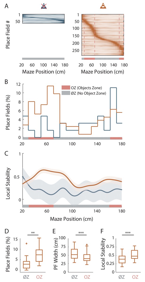
Virtual 3D objects improve spatial coding resolution locally.
(A) Color-coded mean firing rate maps of all place fields recorded in the maze without objects (left) or with objects (right). The color codes for the intensity of the bin’s mean firing rate normalized on the maximal mean firing rate (peak rate) in the recording session. The place cells are ordered according to the position of their peak rate in the track (reward zones excluded). Bottom: The tracks were divided into Objects Zones (OZ, in red on the x-axis) around the objects and No Object Zones (ØZ, in grey on the x-axis) deprived of objects. Red dotted lines depict the boundaries of the OZ in the track with objects. (B) Percentage of On-Track place fields at each spatial bin (10 cm) in the maze with (orange line) and without objects (blue line). (C) Mean local stability index (solid lines)±SEM (shaded bands) for place cells with On-Track fields at each spatial bin in the track with (orange) or without (blue) objects. (D–F) Box plots depicting the mean percentage of place fields per spatial bin (D), the place field width (E) and the local stability index (F) in OZ and ØZ in the maze with objects. Figure 2—source data 1. Source data for Figure 2.
-
Figure 2—source data 1
Source data for Figure 2.
- https://doi.org/10.7554/eLife.44487.008
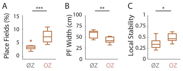
Virtual 3D objects improve spatial coding resolution locally across different recording sessions.
(A–C) Box plots of the mean percentage of place fields per spatial bin (A; ØZ: 3.49 ± 0.40%/10 cm, n = 8 recording sessions; OZ: 7.36 ± 0.82%/10 cm, n = 8 recording sessions; t14 = −4.24, p=0.0008, two-tailed unpaired t-test), the place field width (B; ØZ: 57.1 ± 3.19 cm, n = 8 recording sessions; OZ: 43.2 ± 2.49 cm, n = 8 recording sessions; t14 = 3.46, p=0.0038, two-tailed unpaired t-test) and the local stability index (C; ØZ: 0.36 ± 0.04, n = 8 recording sessions; OZ: 0.50 ± 0.03, n = 8 recording sessions; t14 = −2.53, p=0.02, two-tailed unpaired t-test) in ØZ and OZ in the maze with objects between different recording sessions.
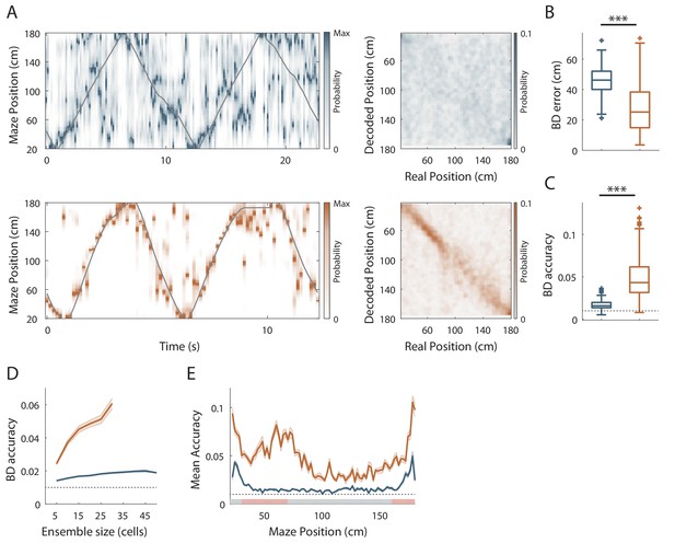
Effect of visual cues on spatial coding resolution at the population level.
(A) Left: Color-coded distribution of the animal position’s probability in the virtual track (the reward zones are excluded) computed using a Bayesian decoder (see Materials and methods) at each time window (500 ms) illustrated during four trials in the maze without (top) and with (bottom) objects. Spike trains of active cells were used to compute the animal position’s probability. For visualization purpose, position probability is normalized by its maximum at each time bin. The real position is indicated with a solid grey line. Right: Confusion matrix between the real (x-axis) and the decoded position (y-axis) for all recording sessions performed on the track without objects (top) or with objects (bottom). (B) Box plots depicting the Bayesian decoding error (BD error) in the maze with and without objects. The BD error was significantly higher in the maze deprived of objects. (C) Box plots depicting the Bayesian decoding accuracy (BD accuracy) in the maze with and without objects. The BD accuracy was significantly higher in the maze with objects. (D) Mean BD accuracy (solid lines)±SEM (shaded bands) as a function of a subset of active cells in the maze with and without objects. (E) Mean BD accuracy (solid lines)±SEM (shaded bands) at each position in the maze with and without objects. The track was divided in two zones: Objects Zone (OZ, in red on the x axis) around the objects and No Object Zone (ØZ, in grey on the x axis) deprived of objects. Note that the decoding accuracy was specifically improved in OZ in comparison to ØZ in the maze with objects.
-
Figure 3—source data 1
Source data for Figure 3.
- https://doi.org/10.7554/eLife.44487.012
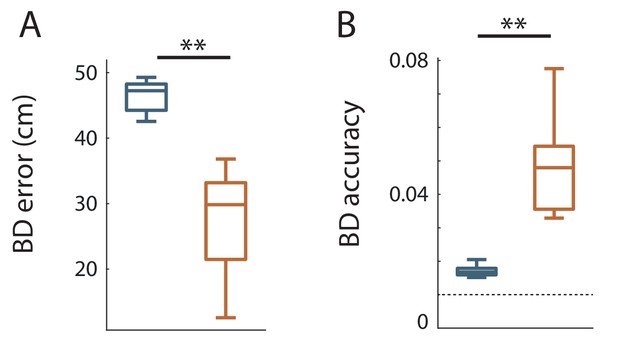
Virtual 3D objects improve hippocampal population coding accuracy across different recording sessions Box plots of the Bayesian decoding error.
(A; BD error; ØT: 46.3 ± 1.20 cm, n = 5 recording sessions; OT: 27.6 ± 3.26 cm, n = 7 recording sessions; Z = 2.76, p=0.0058) and Bayesian decoding accuracy (B; BD accuracy; ØT: 0.017 ± 9×10⁻⁴, n = 5 recording sessions; OT: 0.048 ± 0.005, n = 7 recording sessions; Z = 2.76, p=0.0058) in the maze without (blue) and with (orange) objects.
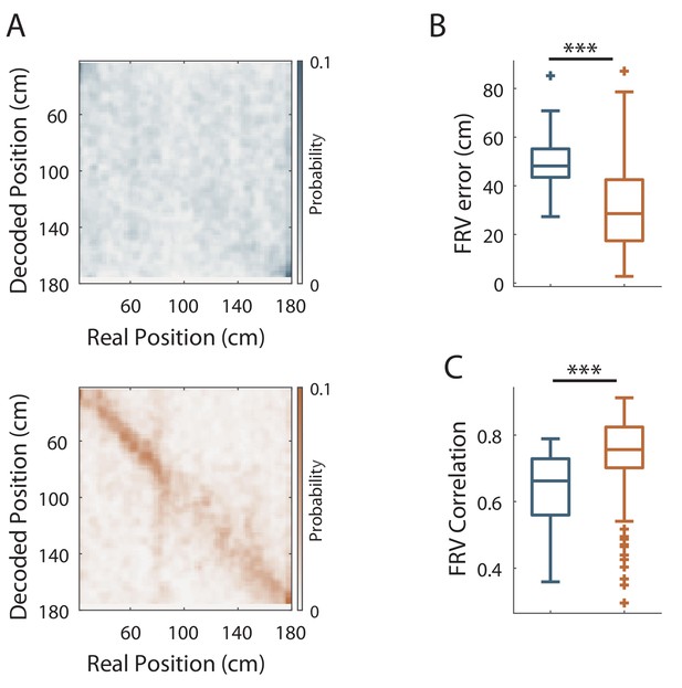
Firing Rate vector decoding in familiar conditions.
(A) Confusion matrix between the real (x-axis) and the decoded position (y-axis) for all recording sessions performed on the track without objects (top, blue) or with objects (bottom, orange). (B) Box plots depicting the Firing Rate Vector decoding error (FRV error) in the maze with (orange) and without (blue) objects. (C) Box plots depicting the Firing Rate Vector decoding accuracy (FRV correlation) in the maze with and without objects.
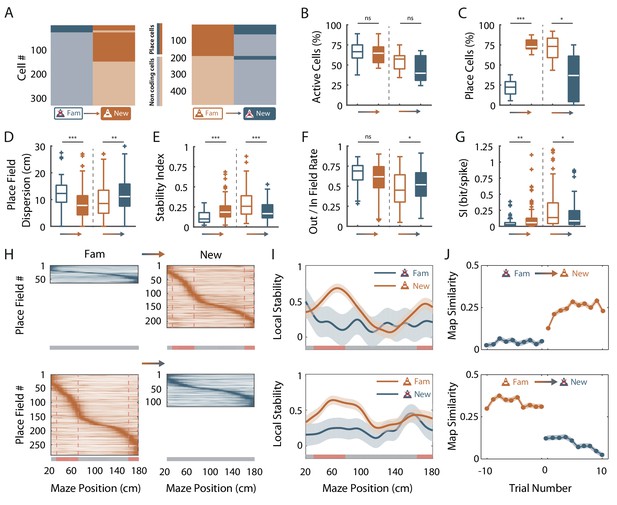
Fast dynamics of spatial coding resolution tuning upon objects manipulation.
(A) Mosaic plots representing the cells classified as place cells (darker orange and blue) or non-coding cells (i.e. silent or active non-coding, lighter orange and blue) in the familiar and the new mazes. (B–G) Box plots comparing familiar (empty box) and new mazes (filled box) conditions. Two pairs of box plots are illustrated; Left: comparison between the familiar maze without objects (blue, ØTfam) and the new maze with objects (orange, OTnew). Right: comparison between the familiar maze with objects (orange, OTfam) and the new maze without objects (blue, ØTnew). A gradient color arrow shows the way of the transition. Plots show the percentage of active cells (B), the percentage of place cells (C), the Out/In field firing rate (D), the spatial information (SI; E) and the stability index (G). (H) Color-coded mean firing rate maps of place fields recorded in the familiar and new mazes. The color codes for the intensity of the firing rate normalized by the peak rate. The place fields are ordered according to the position of their peak rate in each track (the reward zones are excluded). The tracks were divided into Objects Zones (OZ, in red on the x-axis) around the objects and No Object Zones (ØZ, in grey on the x-axis) deprived of objects. Red dotted lines depict the boundaries of the OZ in the track with objects. (I) Mean local stability index (solid orange or blue lines)±SEM (blue or orange shaded areas) at each spatial bin in the familiar and new mazes (top: from ØTfam to OTnew; bottom: from OTfam to ØTnew). (J) Map similarity (see Materials and methods) for 10 trials before and 10 trials after the experimental manipulation (indicated by 0) for ØTfam to OTnew (top) and for OTfam to ØTnew condition (bottom).
-
Figure 4—source data 1
Source data for Figure 4.
- https://doi.org/10.7554/eLife.44487.016

Spatial coding resolution adaptation upon objects manipulations is already visible during the first session in the new condition Box plots comparing familiar (empty boxes, all recording sessions) and new (filled boxes, first recording session) conditions upon objects manipulation.
Two pairs of box plots are illustrated; Left: comparison between the familiar condition without objects (blue, ØTfam) and the new condition with objects (orange, OTnew). Right: comparison between the familiar maze with objects (orange, OTfam) and the new maze without objects (blue, ØTnew). A gradient color arrow shows the direction of the transition. Plots show the place field spatial dispersion (A; ØTfam vs OTnew: Z = 2.85, p=0.0043, two-tailed WRS test; OTfam vs ØTnew: Z = −2.62, p=0.008, two-tailed WRS test), the stability index (B; ØTfam vs OTnew: Z = −4.91, p<10−6, two-tailed WRS test; OTfam vs ØTnew: Z = 4.41, p<10−4, two-tailed WRS test), the out/in field firing (C; ØTfam vs OTnew: Z = 3.34, p=0.001, two-tailed WRS test; OTfam vs ØTnew: Z = −2.71, p=0.006, two-tailed WRS test) and the spatial information (SI; D; ØTfam vs OTnew: Z = −3.94, p<10−4, two-tailed WRS test; OTfam vs ØTnew: Z = 2.74, p=0.006, two-tailed WRS test).
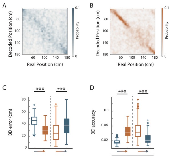
Virtual 3D objects modulation of hippocampal population coding accuracy upon objects manipulation.
(A–B) Confusion matrix between the real (x-axis) and the decoded position (y-axis) for all new recording sessions performed on the track without objects (A, blue) or with objects (B, orange). (C–D) Box plots comparing Bayesian decoding in familiar (empty boxes) and new (filled boxes) conditions upon objects manipulation. Two pairs of box plots are illustrated; Left: comparison between the familiar condition without objects (blue, ØTfam) and the new condition with objects (orange, OTnew). Right: comparison between the familiar maze with objects (orange, OTfam) and the new maze without objects (blue, ØTnew). A gradient color arrow shows the direction of the transition. Plots show the Bayesian decoding error (C; ØTfam: 46.3 ± 0.70 cm, n = 180 trials vs OTnew: 30.7 ± 1.09 cm, n = 86 trials; t264 = 12.4, p<10−27; two-tailed unpaired t-test; OTfam: 27.1 ± 0.94 cm, n = 249 trials vs ØTnew: 37.6 ± 1.18 cm, n = 175 trials; Z = −6.58, p<10−35, two-tailed WRS test) and the Bayesian decoding accuracy (D; ØTfam: 0.017 ± 3.8×10⁻⁴, n = 180 trials vs OTnew: 0.046 ± 1.8×10⁻³, n = 86 trials; Z = −12.6, p<10−35, two-tailed WRS test; OTfam: 0.05 ± 1.5×10⁻³, n = 249 trials vs ØTnew: 0.026 ± 1.1×10⁻³, n = 175 trials; Z = 10.6, p<10−25, two-tailed WRS test).
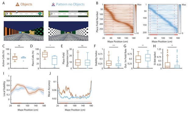
Effects of 2D wall patterns on hippocampal spatial coding resolution.
(A) Schema (top) and picture (bottom) representing the original maze with objects (orange, left) and a maze with patterns on the walls but no objects (PØT; ligth blue, right). (B) Color-coded mean firing rate maps for all place fields recorded in the original maze with objects (orange, left) and on the PØT maze (light blue, right). The color codes for the intensity of the firing rate normalized by the peak rate. The place fields are ordered according to the position of their peak rate in each track (the reward zones are excluded). The tracks were divided into Objects Zones (OZ, in red on the x-axis) around the objects and No Object Zones (ØZ, in grey on the x-axis) deprived of objects. Red dotted lines depicts the boundaries of the OZ. (C–H) Box plots representing in the original (orange) and pattern no object (light blue) mazes the percentage of active cells (C), the percentage of place cells (D), the place field dispersion (E), the stability index (F), the out/in field rate (G) and the spatial information (SI; H). (I) Mean local stability index (solid orange or light blue lines)±SEM (orange or light blue shaded bands) at each position’s bin in the original (orange) and pattern no object (light blue) mazes. (J) Mean BD accuracy (solid lines)±SEM (shaded bands) at each spatial bin in the original maze with objects (orange) or in the pattern no object maze (light blue).
-
Figure 5—source data 1
Source data for Figure 5.
- https://doi.org/10.7554/eLife.44487.018
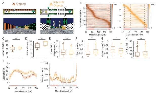
Spatial coding resolution in a visually enriched environment .
(A) Schema (top) and picture (bottom) representing the original maze with objects (left) and a visually enriched maze with objects (right). (B) Color-coded mean firing rate maps for all place fields recorded in the original maze with objects (orange, left) and on the visually rich maze with objects (yellow, right). The color codes for the intensity of the firing rate normalized by the peak rate. The place fields are ordered according to the position of their peak rate in each track (the reward zones are excluded). The tracks were divided into Objects Zones (OZ, in red on the x-axis) around the objects and No Object Zones (ØZ, in grey on the x-axis) deprived of objects. Red dotted lines depicts the boundaries of the OZ. (C–H) Box plots representing in the original (orange) and pattern no object (light blue) mazes the percentage of active cells (C), the percentage of place cells (D), the place field dispersion (E), the stability index (F), the out/in field rate (G) and the spatial information (SI; H). (I) Mean local stability index (solid orange or yellow lines)±SEM (orange or yellow shaded bands) at each position’s bin in the original (orange) and visually rich (yellow) mazes. (J) Mean BD accuracy (solid lines)±SEM (shaded bands) at each spatial bin in the original maze with objects (orange) or in the visually rich maze with objects (yellow).
-
Figure 6—source data 1
Source data for Figure 6.
- https://doi.org/10.7554/eLife.44487.020
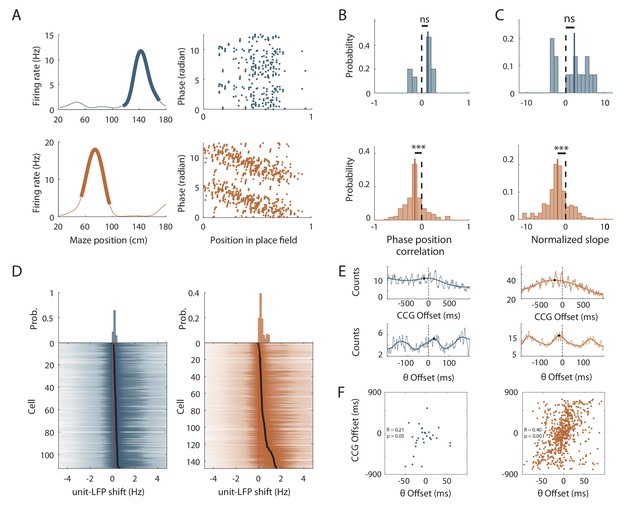
Effects of local cues on hippocampal temporal coding resolution .
(A) Left: Mean firing rate maps of representative CA1 place cells with place fields highlighted by a bold line (left) recorded in the maze without objects (top, only spatially stable trials see Materials and methods section) and with objects (bottom). Right: spikes phase (radian) versus position in the corresponding place fields. (B–C) Distribution of significant phase position correlation (B) and slopes (C) in the condition without objects (top; correlation) and with objects (bottom). The median of the distribution is indicated by a bold line and 0 by a dotted line. (D) Color-coded cross-correlogram between the power spectra of neuronal spikes and LFP for each theta-modulated cell recorded on the maze without (bottom left, blue) and with (bottom right, orange) objects. Black dots indicate the maximum of each cross-correlation. Each cross-correlation is normalized by its maximum. Top: Distribution of the maximum cross-correlations used to quantify the frequency shift for all the cells. (E) Examples of cross-correlograms computed for two pairs of place cells with overlapping place fields at the behavioral (top) or theta time scale (bottom, see Materials and methods) in order to quantify Cross-Correlogram (CCG) and theta Offsets respectively in no object (blue; left) or object (orange; right) conditions. (F) Relationship between ‘CCG’ and ‘theta’ offsets in the cross-correlograms of all the spikes in overlapping place fields of neuron pairs recorded in no object (top; blue) and object condition (bottom; orange).
-
Figure 7—source data 1
Source data for Figure 7.
- https://doi.org/10.7554/eLife.44487.025
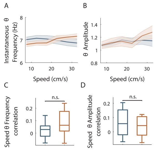
Speed modulation of LFP theta frequency and amplitude in OT and ØT.
(A–B) Mean theta frequency (A) or amplitude (B) across all recording sessions as a function of animal speed (bin: 5 cm/s). (C–D) Box plots of the correlation between theta frequency (C) or amplitude (D) vs speed for individual sessions.
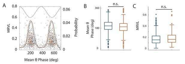
Theta modulation of spikes in OT and ØT.
(A) Mean theta phase plotted against strength of phase locking (Mean Resultant Vector Length: MRLV) for all theta modulated cells (p<0.05, Rayleigh Test) in OT (orange) and ØT (blue). Solid lines: probability distribution of the preferred theta phase for the two conditions. Black line: illustrative theta cycle (B) Box plots of the mean theta phase for OT(orange) and ØT (blue) conditions (C) Box plots of the Mean Resultant Vector Length in OT(orange) and ØT (blue) conditions.
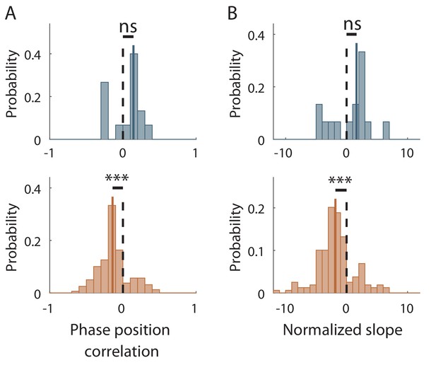
Effect of objects on theta phase precession estimated with a waveform-based approach Distribution of significant phase position correlation (left) and slopes (right) in the condition without objects (top, blue) and with (bottom, orange) when theta phase was detected using a waveform-based approach which takes into account theta waves asymmetry.
The median of the distribution is indicated by a bold line and 0 by a dotted line. (A) The correlation between phase and position was significantly different from zero for place cells recorded in the track with objects (r = −0.14 ± 0.016, n = 159 fields; p<10−13, one sample sign-test) but not for those recorded in the track without objects (r = 0.14 ± 0.05, n = 15 fields; p=0.30, one sample sign-test). (B) Phase precession slopes (calculated on normalized place field sizes) were negative and significantly different from 0 for cells recorded in the track with objects (−1.83 ± 0.24 rad/U, n = 159 fields; p<10−13, one sample sign-test) but not in the track without objects (1.63 ± 0.84 rad/U, n = 15 fields; p=0.3, one sample sign-test).
Additional files
-
Supplementary file 1
Details of the recorded units and animal behavior per recording session in different mazes.
TA: Track Active. Rw.: Number of rewards.
- https://doi.org/10.7554/eLife.44487.026
-
Supplementary file 2
Details of place cells' firing properties per recording session in different mazes.
- https://doi.org/10.7554/eLife.44487.027
-
Transparent reporting form
- https://doi.org/10.7554/eLife.44487.028


