Linking spatial patterns of terrestrial herbivore community structure to trophic interactions
- Mammal Research Institute, Polish Academy of Sciences, Poland
Figures
Figure 1
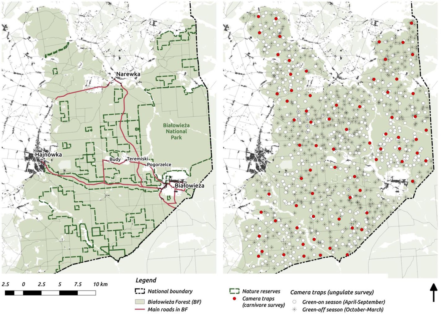
Maps of the study area (left) and camera trapping sampling design (right).
On the study area map we marked the major settlements connected by public roads open for cars.
Figure 2
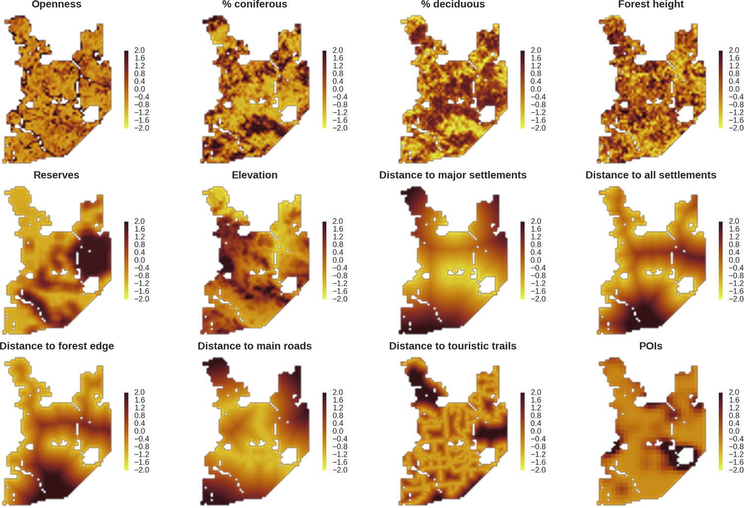
Maps of candidate landscape-scale covariates for the ungulate and carnivore models representing environmental and human-related landscape gradients.
All covariates were scaled and zero-centered prior to modelling. POIs – density of tourist infrastructure. When selecting covariates for the final models we ensured that the Pearson correlation value for all pairs of included covariates was lower than 0.7 (Appendix 1—figure 1).
Figure 3
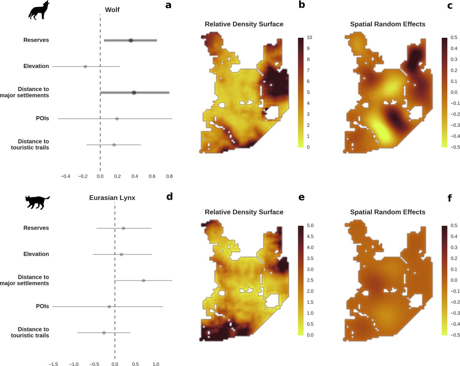
Spatial distribution of large carnivores is determined by human activity.
(a, d) Estimated parameters for the wolf and lynx models, (b, e) maps of the predicted variation in their landscape use (relative density surfaces) and (c, f) fitted spatial random effects (SRE). Specifically, panels (b) and (e) present the spatial predictions for the parameter , which is the expected number of individuals using a given landscape grid cell (25 ha pixel) during the sampling period (see the general and formal description of the model in the Materials and methods section). The fitted values of SRE are deviations from 0 at log-scale. The SRE captured all spatial variation not explained by the covariates included in the model, indicating parts of the landscape for which higher (“hot-spots”) or lower (“cold-spots”) activities of species were observed in the data than was predicted by the “fixed” part of the model. On panels (a) and (b) we additionally marked in bold the credibility intervals (quantile based) at which the estimated parameter values differed from 0 (for the level 2.5–97.5%, there is a 0.95 probability that the true parameter value lies within this range). The full posterior distribution for each parameter, together with its numerical description can be found in Appendix 1—figures 26–27).
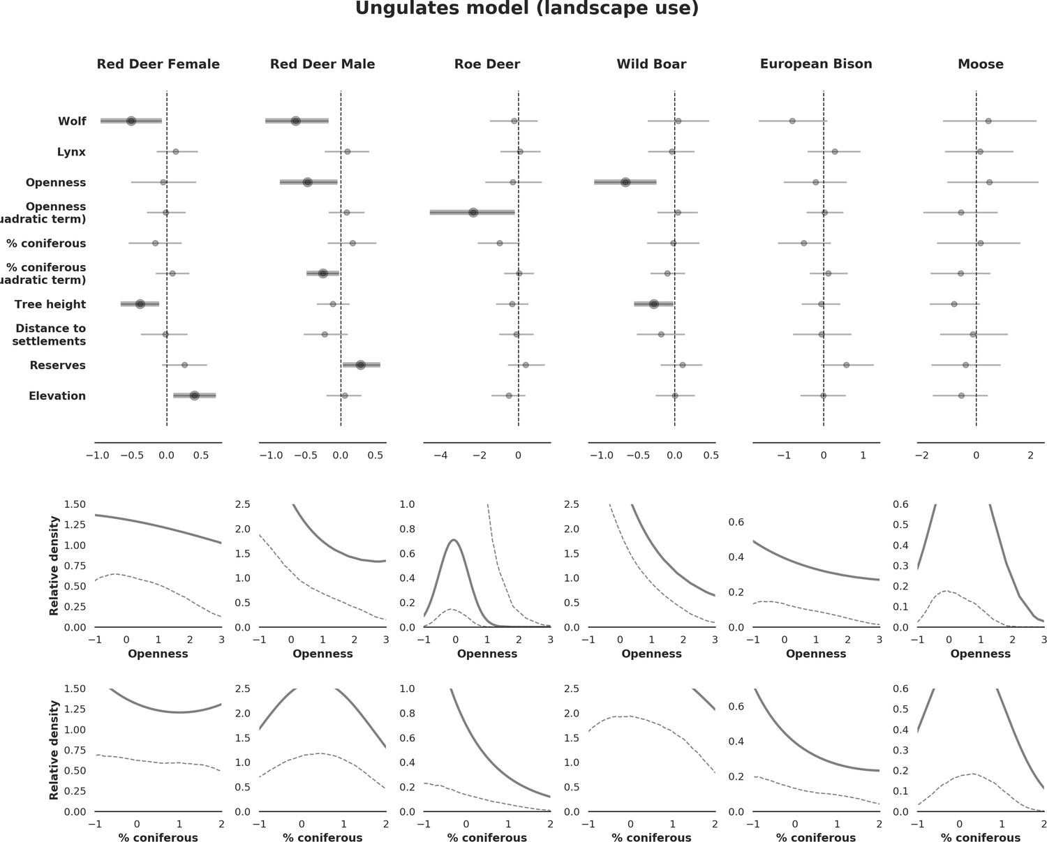
Figure 4
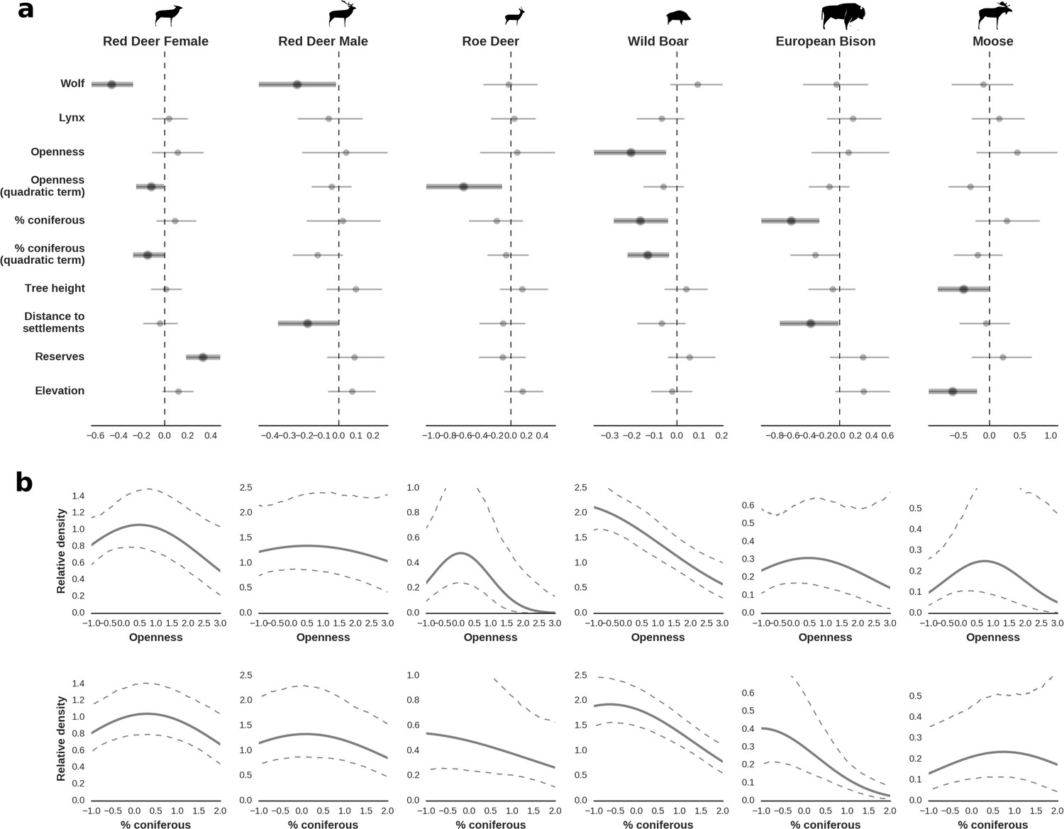
Spatial distribution of each ungulate species was related to a unique combination of bottom-up and top-down factors.
(a) Estimated effects of covariates explaining the spatial variation in the parameter , which is the expected number of individuals using a given landscape grid cell (25 ha pixel) during the sampling period (i.e. the relative density; see the general and formal description of the model in the Materials and methods section). In bold, we marked the credibility intervals (quantile based) at which the estimated parameter values differed from 0 (for the level 2.5–97.5%, there is 0.95 probability that the true parameter value lies within this range). The full posterior distribution for each parameter, together with its numerical description can be found in Appendix 1. (b) For easier interpretation of the effects of landscape openness and percentage share of coniferous species (together with their quadratic terms and assuming an average level for the other covariates), we plotted predictions of the relative density for each species and for each variable. The values of the covariates were scaled and zero-centered before making predictions; thus 0 corresponds to the average value of a given covariate. The full posterior distribution for each parameter, together with its numerical description can be found in Appendix 1—figures 14–25).
Figure 5
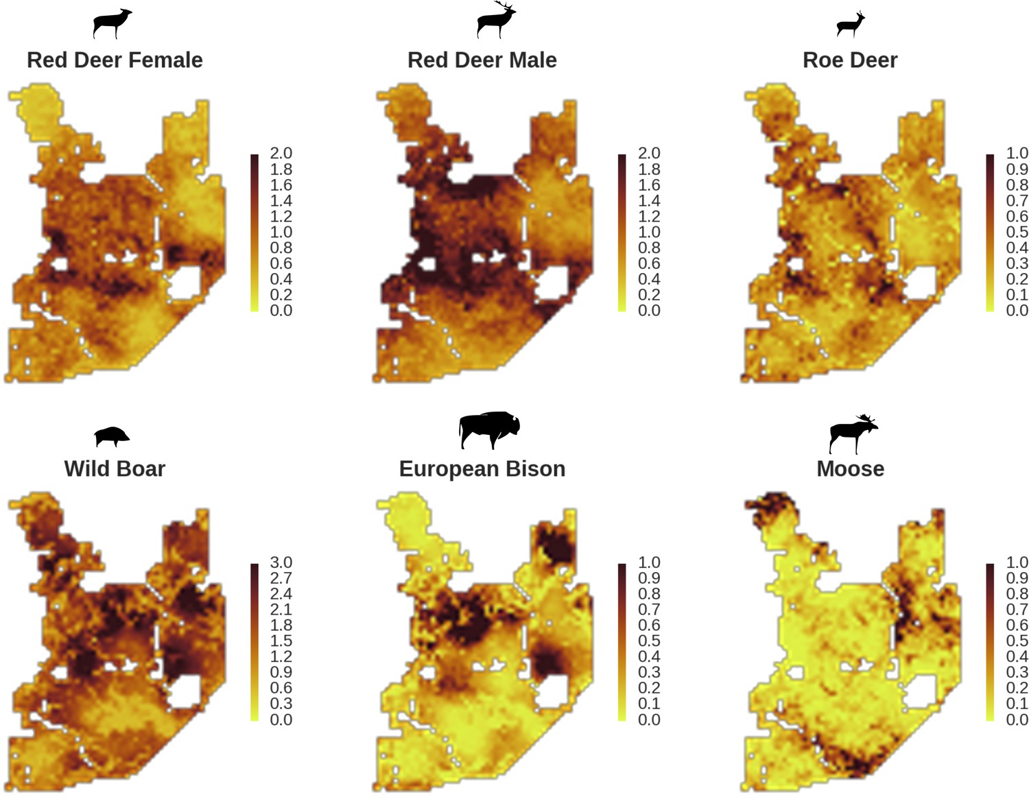
Only red deer (the major wolf prey) showed a negative spatial association with parts of the landscape intensively used by wolves, whereas distributions of other species were shaped by bottom-up factors.
The maps show substantial variation in predicted landscape use for the five studied ungulate species (relative density surfaces). Specifically, this figure presents the spatial predictions for the parameter which is the expected number of individuals using a given landscape grid cell (25 ha pixel) during the sampling period (see the general and formal description of the model in the Materials and methods section). The predictions are based on the parameter estimates presented in Figure 3 and include the spatial random effects (see Figure 4).
Figure 6
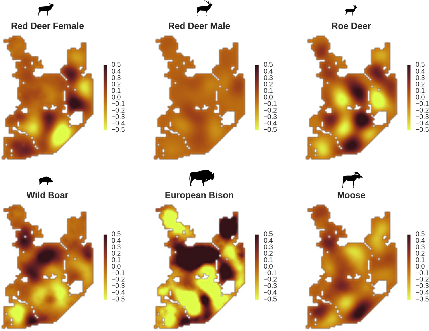
All ungulate species except red deer males showed some level of remaining spatial auto-correlation not explained by the raster covariates included in the models.
The maps show the fitted spatial random effects (SRE) for the models of five studied ungulate species. The SRE are deviations from 0 at log-scale. The SRE captured all spatial variation not explained by covariates included in the model, indicating parts of the landscape for which higher (‘hot-spots’) or lower (‘cold-spots’) activity of species was observed in the data than predicted by the ‘fixed’ part of the model. The SRE were particularly large for the bison, whose spatial distribution in BF is strongly influenced by supplementary winter feeding and the use of open areas outside the forest during the year.
Figure 7
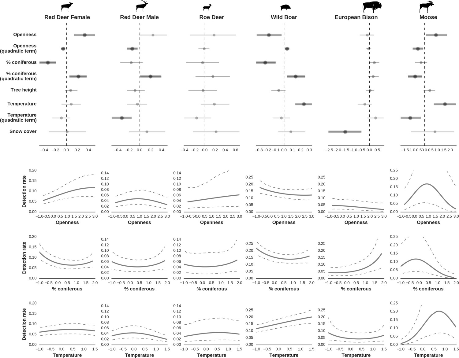
Factors influencing detection rates of ungulate species.
(a) Estimated effects of covariates explaining the variation in the parameter , which is the expected (daily) detection (trapping) rate at a single camera trap site (see the general and formal description of the model in the main text in the Materials and methods section). The spatial covariates were calculated at a pixel resolution of 100 m (1 ha) and the temporal covariates were calculated as the average value for the whole period of camera trapping at a given location. In bold, we have marked the credibility intervals (quantile based) at which the estimated parameter values differ from 0 (for the level of 2.5–97.5 %, there is a 0.95 probability that the true parameter value lies within this range). The full posterior distribution for each parameter, together with its numerical description can be found in Appendix 1. (b) For easier interpretation of the effects of canopy openness, the percentage share of coniferous species and temperature (together with their quadratic terms and assuming an average level for other covariates), we plotted predictions of the detection rate for each species and for each variable. The values of the covariates were scaled and zero-centered before making predictions; thus 0 corresponds to the average value of a given covariate. The full posterior distribution for each parameter, together with its numerical description can be found in (Appendix 1—figures 14–25).
Figure 8

There was substantial spatial variation in the structure of the ungulate community, as indicated by the weak spatial associations between species.
The pairwise spatial overlap between the studied ungulate species is presented as the Pearson correlation heatmap of their relative density surfaces predicted by the models (a) and fitted spatial random effects (b).
Figure 9
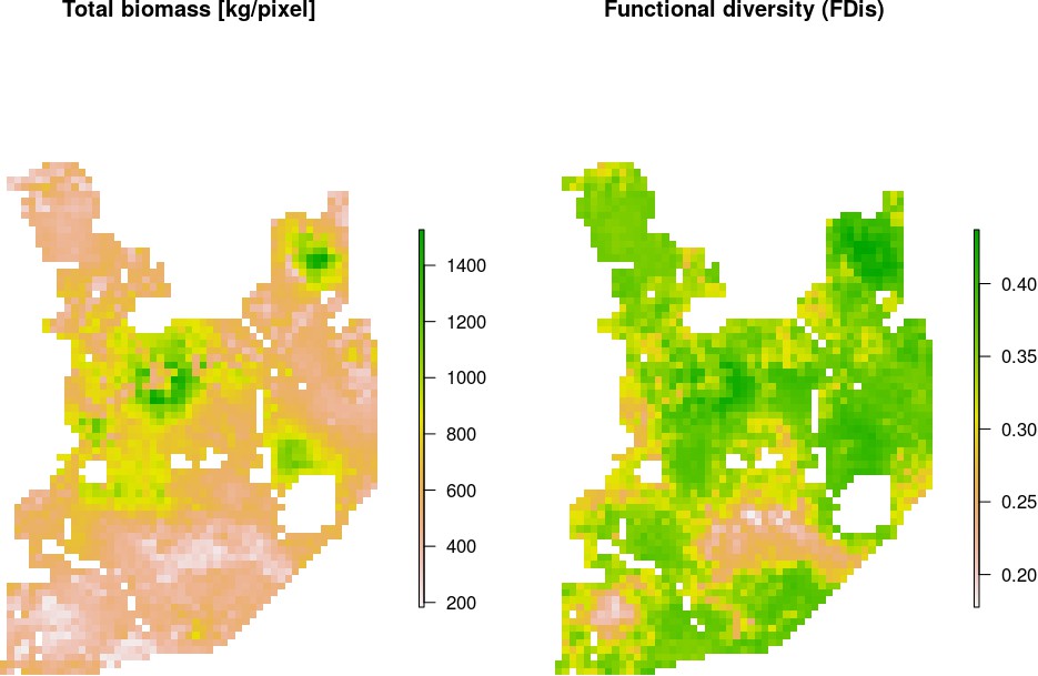
Maps of estimated total biomass [kg/pixel] and functional diversity (FDis).
Both variables, together with species-specific biomass raster layers, were used in the hierarchical clustering analysis. Interestingly, the lowest values of both parameters were largely associated with coniferous-dominated tree stands at higher elevations (compare with Figure 2), often re-planted after extensive clear-cuts from the past and belonging to the least productive parts of this landscape (Faliński and Falińska, 1986; Kwiatkowski, 1994).
Figure 10
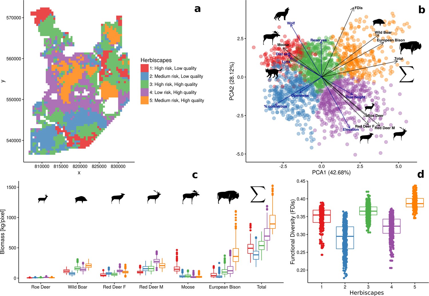
Spatial variation and functional diversity of a herbivore community within a temperate forest herbivome, decomposed into landscape-scale herbivory regimes – herbiscapes.
(a) The spatial distribution of the five identified clusters (‘herbiscapes’) based on hierarchical clustering on the principal components analysis. (b) The distribution of identified clusters in the space of the first two principal components. (c) Tukey-like boxplot comparing the species-specific and total biomass in each of the identified clusters. (d) Tukey-like boxplot comparing the functional diversity index (FDis) of the ungulate community between the identified clusters. The boxplots show median values and the lower and upper hinges correspond to the first and third quartiles. The colors of clusters are consistent amongst all figures. Each data point on panel (b) corresponds to a 25 ha pixel mapped on figure (a). On panel (b), for ease of interpretation, we additionally plotted (blue arrows) the major environmental and risk-related gradients in the study area which were used as covariates in the ungulate models.
Figure 11
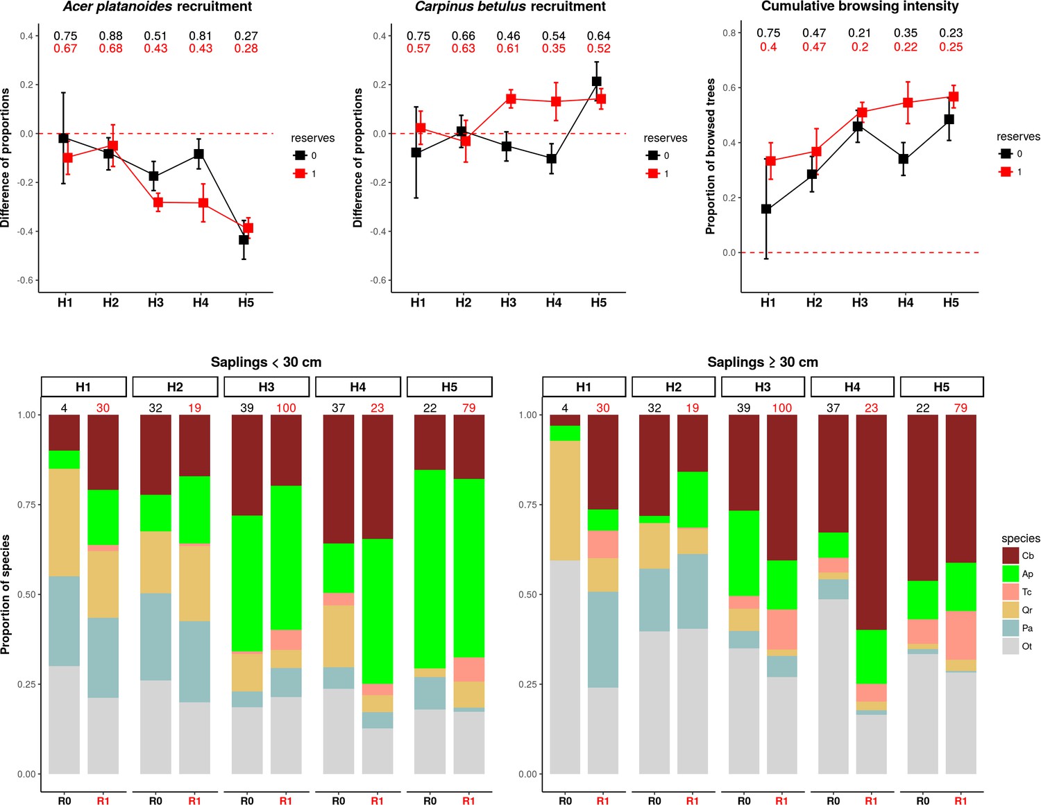
The patterns of browsing intensity and the composition of regenerating tree species differ between herbiscapes and between the protected and managed parts of the BF landscape.
(a, b) The mean differences between the two tree height classes (saplings < 30 cm and ≥30 cm) in the proportional shares of Acer platanoides (Acer) and Carpinus betulus (Carpinus). The numbers on top of both figures are the proportions of plots without a single individual of each species. (c) The cumulative browsing intensity index, expressed as the proportion of browsed individual trees out of all tree saplings ≥ 30 cm. The numbers on top of this figure are the proportions of plots with no browsing. Panels (a), (b) and (c) show the values predicted by the fitted linear models with two interacting factors: herbiscape (six levels) and reserves (two levels coded as 0: unprotected areas and 1: protected areas). The error bars are standard errors of the mean. (d) The mean proportions of selected tree species (saplings < 30 cm and ≥30 cm) out of the entire pool of the main regenerating trees recorded at the sampled plots, showed for the herbiscapes and protected (R1) and unprotected (R0) areas separately. The value on top of each stacked bar is the number of plots used to calculate the mean proportion. Cb: Carpinus betulus, Ap: Acer platanoides, Tc: Tilia cordata, Qr: Quercus robur, Pa: Picea abies, Ot: other species (Betula pendula, Sorbus aucuparia, Fraxinus excelsior, Alnus glutinosa, Populus tremula, Pinus sylvestris, Ulmus).
Figure 12
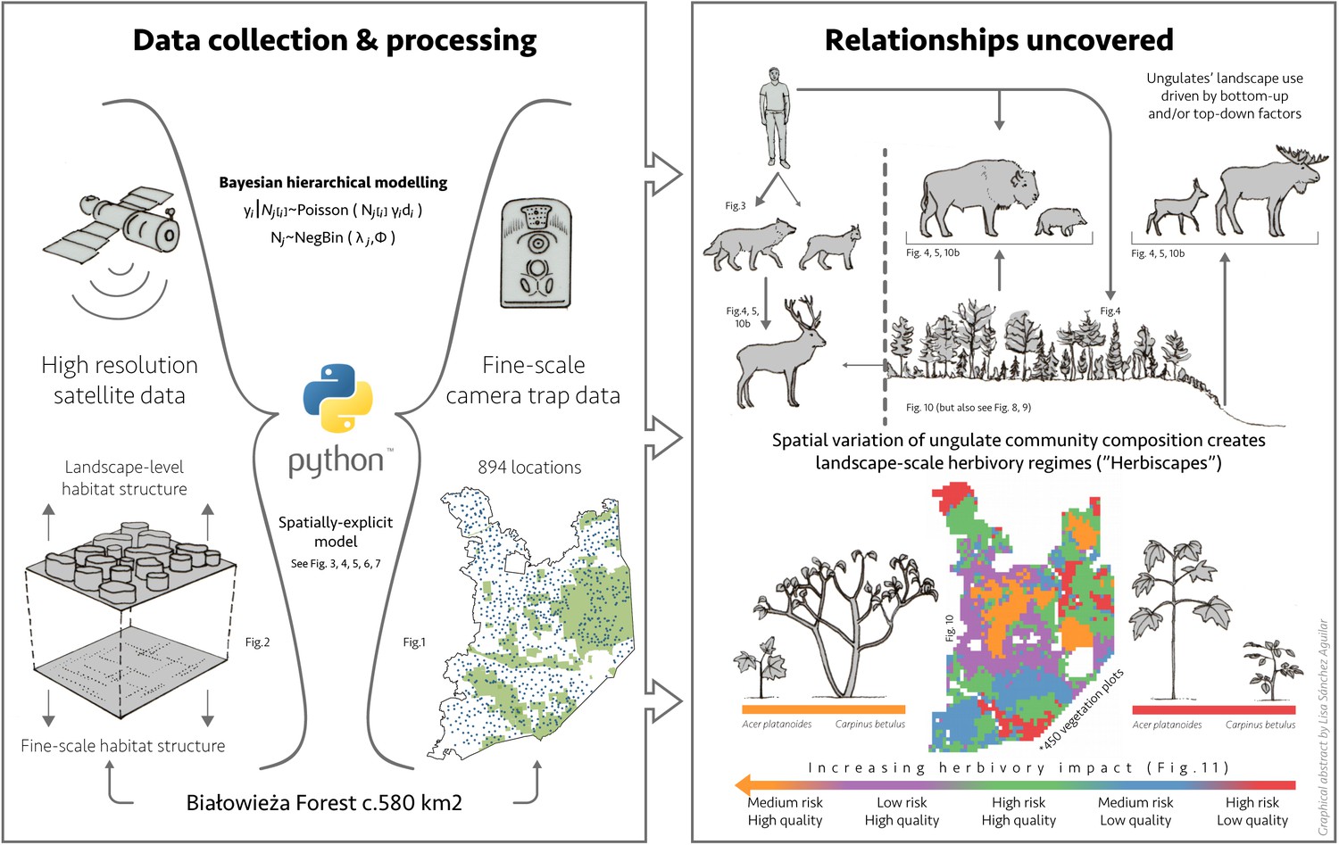
Graphical abstract presenting the steps taken to reveal the relationships uncovered in this study.
Image credit: Lisa Sánchez Aguilar
Figure 13
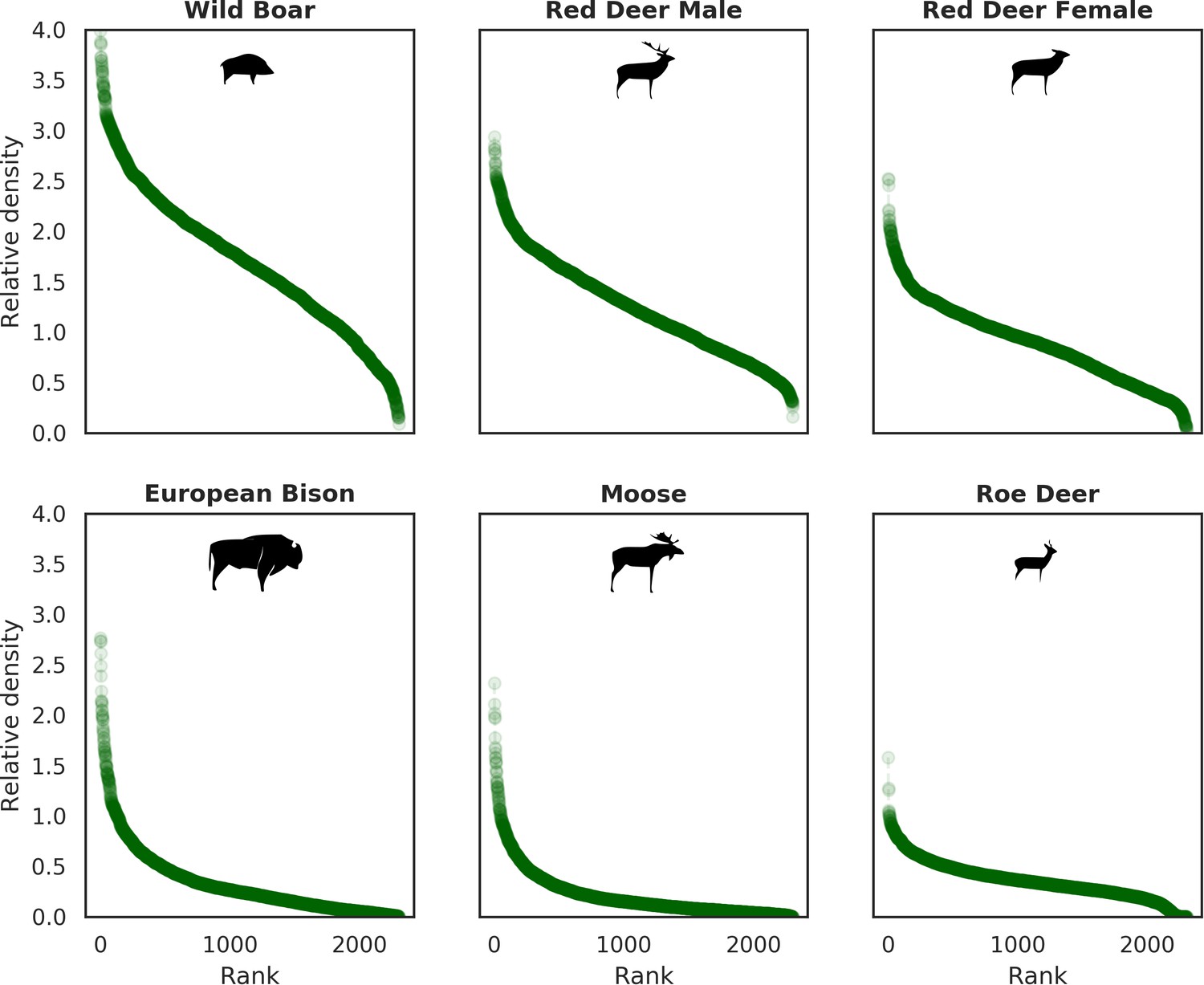
Ranked relative densities predicted for all ungulate species and for each 25 ha landscape pixel.
All plots follow a characteristic shape of a hollow or sigmoidal curve (Brown et al., 1995; Rocchini and Neteler, 2012) indicating a non-uniform, heterogenous distribution of all studied species.
Figure 14
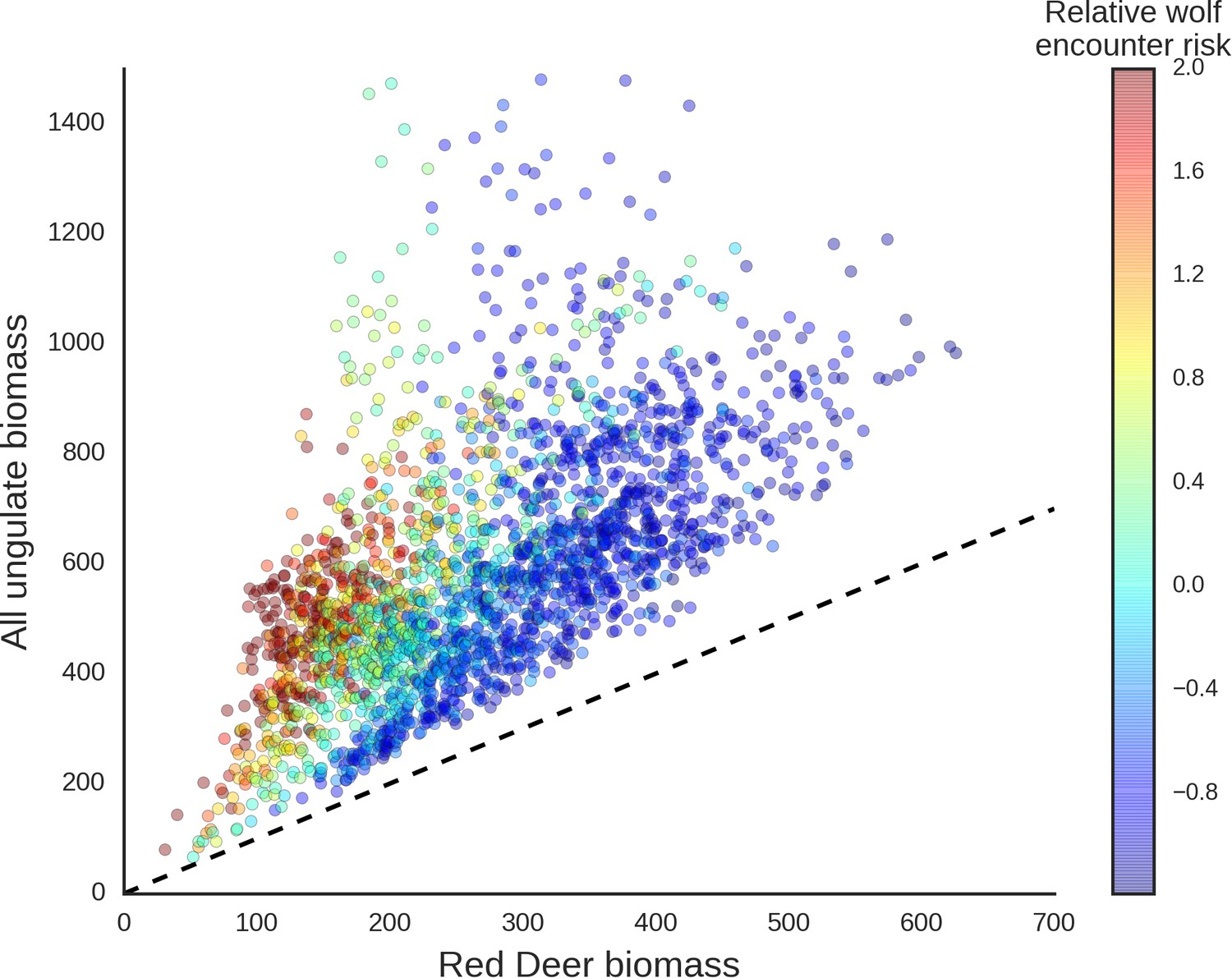
Scatter plot showing how wolves, by affecting the spatial distribution of red deer, re-structured the composition of the entire community of large herbivores.
The predicted biomass of red deer (both sexes, X axis) is shown as a share of the total biomass of the entire community of ungulates. Each dot on the plot is a 25 ha landscape pixel. In color, we marked relative wolf encounter risk (scaled values of the parameter ) as predicted by the model fitted to the wolf camera trapping data. We interpreted the parameter as large carnivore space use intensity and assumed that from a prey perspective, is proportional to the predator encounter rate. The dashed line is a reference line indicating the y=x relationship.
Appendix 1—figure 1
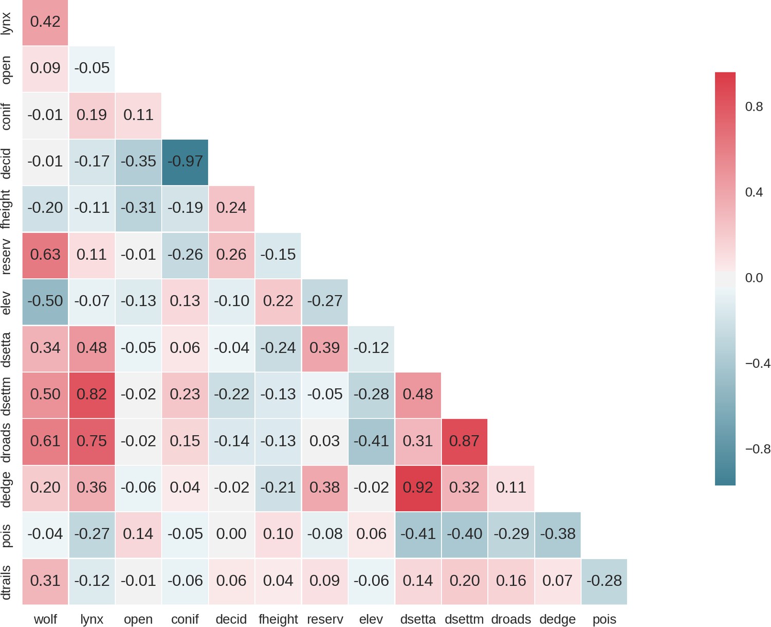
Heatmap of pairwise Pearson correlation values of all candidate landscape-scale covariates for the ungulates models; wolf: predicted use of the landscape by the wolf, lynx: predicted use of the landscape by the lynx, open: landscape openness, conif: % share of coniferous tree species, decid: % share of deciduous tree species, fheight: forest height, reserv: density of protected areas, elev: elevation, dsetta: distance to all settlements, dsettm: distance to major settlements, droads: distance to main roads, dedge: distance to forest edge, pois: density of tourist infrastructure.
When selecting covariates for the final models we ensured that the Pearson correlation value for all pairs of included covariates was lower than 0.7.
Appendix 1—figure 2
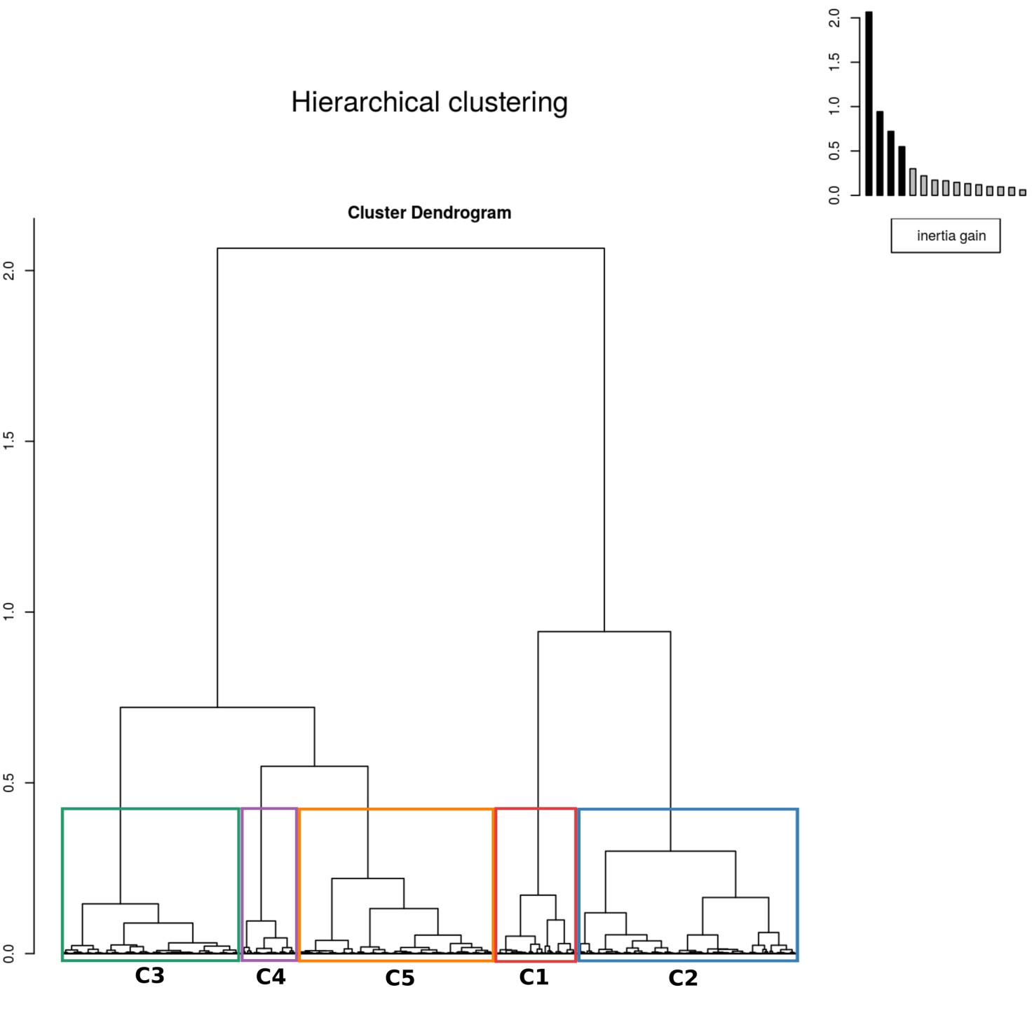
The results of hierarchical clustering on the principal component analysis.
The five clusters were identified by assessing the inertia (i.e. change in within cluster homogeneity) gained by cutting the tree at different levels and the ecological interpretability of the resulting clusters. The colors of the clusters correspond to those in Figure 10 in the main text.
Appendix 1—figure 3
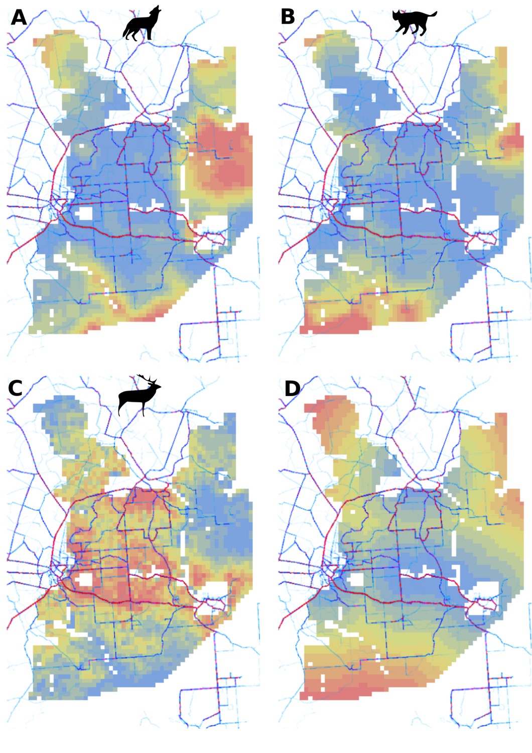
Spatial patterns of human activity in Białowieża Forest derived from the publicly available world-wide data provided by STRAVA (https://www.strava.com/heatmap) combined with (A) predicted use of the landscape by the wolf, (B) predicted use of the landscape by the lynx, (C) predicted use of landscape by the red deer (both sexes) and (D) distance to major settlements used in the models for both large carnivores.
The dark-red thick lines indicate high human activity and the light-blue thin lines indicate low human activity. For (A), (B) and (C) the color gradient from blue to red corresponds to the gradient from low to high use of the landscape by the presented species.
Appendix 1—figure 4
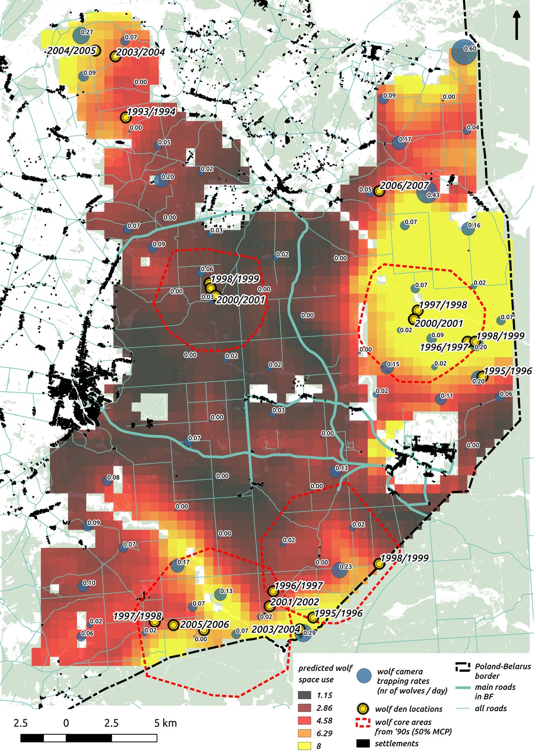
Comparison of predictions of wolf space use with existing radio-tracking data from collared wolves in Białowieża Forest (period 1994–1999, Jędrzejewski et al., 2007) and observations of known den locations (period 1993–2007, MRI PAS unpublished data).
In the background we plotted the raster map of wolf space use predicted by our model together with the raw camera trapping data (‘bubbles’ with trapping rates at each location). On top of it we plotted two datasets: 1) the locations of the core areas (dashed red circles) of the annual territories of the four wolf packs present in the area (50% MCP based on telemetry) and 2) den locations.
Appendix 1—figure 5
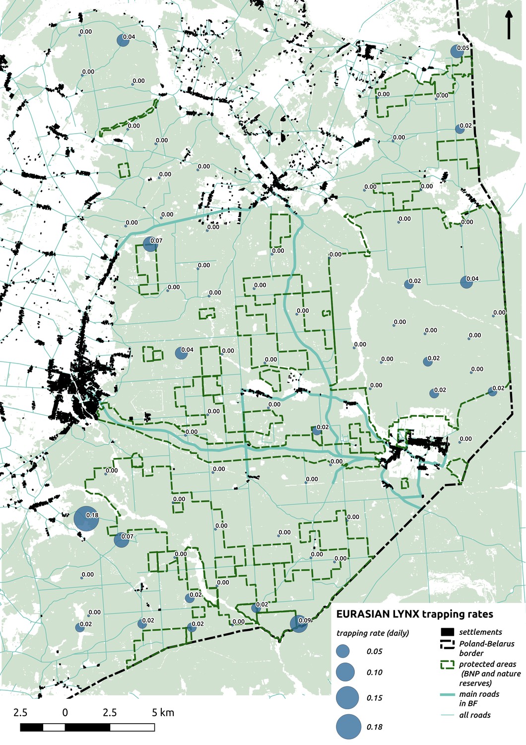
Bubble plot presenting raw camera trapping data for lynx collected during the carnivore survey.
Each bubble is a camera trap location and its size is proportional to the daily trapping rate (i.e. no. of individuals observed/no. of days).
Appendix 1—figure 6
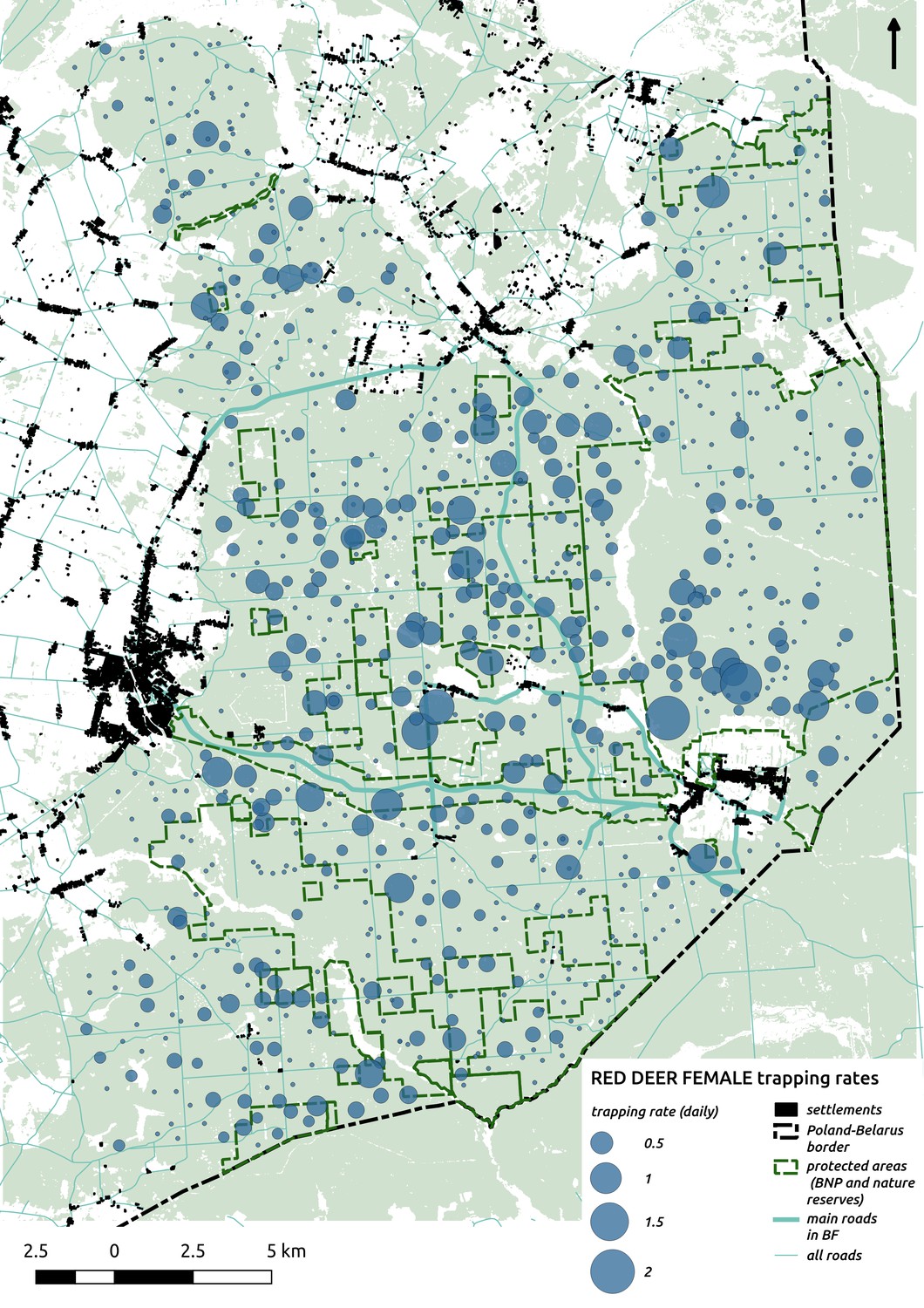
Bubble plot presenting raw camera trapping data for red deer female collected during the ungulate survey.
Each bubble is a camera trap location and its size is proportional to the daily trapping rate (i.e. no. of individuals observed/no. of days).
Appendix 1—figure 7
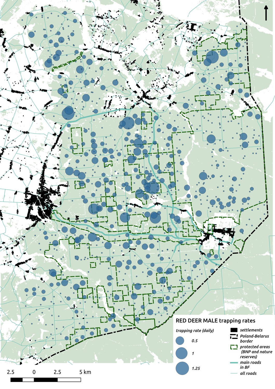
Bubble plot presenting raw camera trapping data for red deer male collected during the ungulate survey.
Each bubble is a camera trap location and its size is proportional to the daily trapping rate (i.e. no. of individuals observed/no. of days).
Appendix 1—figure 8
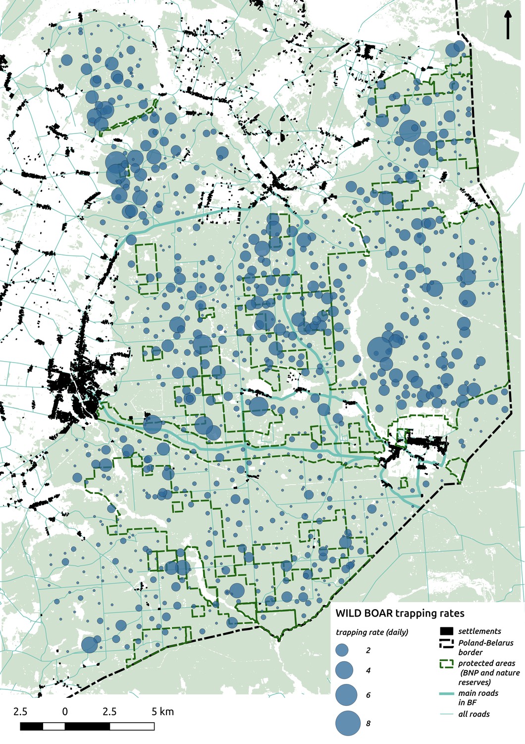
Bubble plot presenting raw camera trapping data for wild boar collected during the ungulate survey.
Each bubble is a camera trap location and its size is proportional to the daily trapping rate (i.e. no. of individuals observed/no. of days).
Appendix 1—figure 9
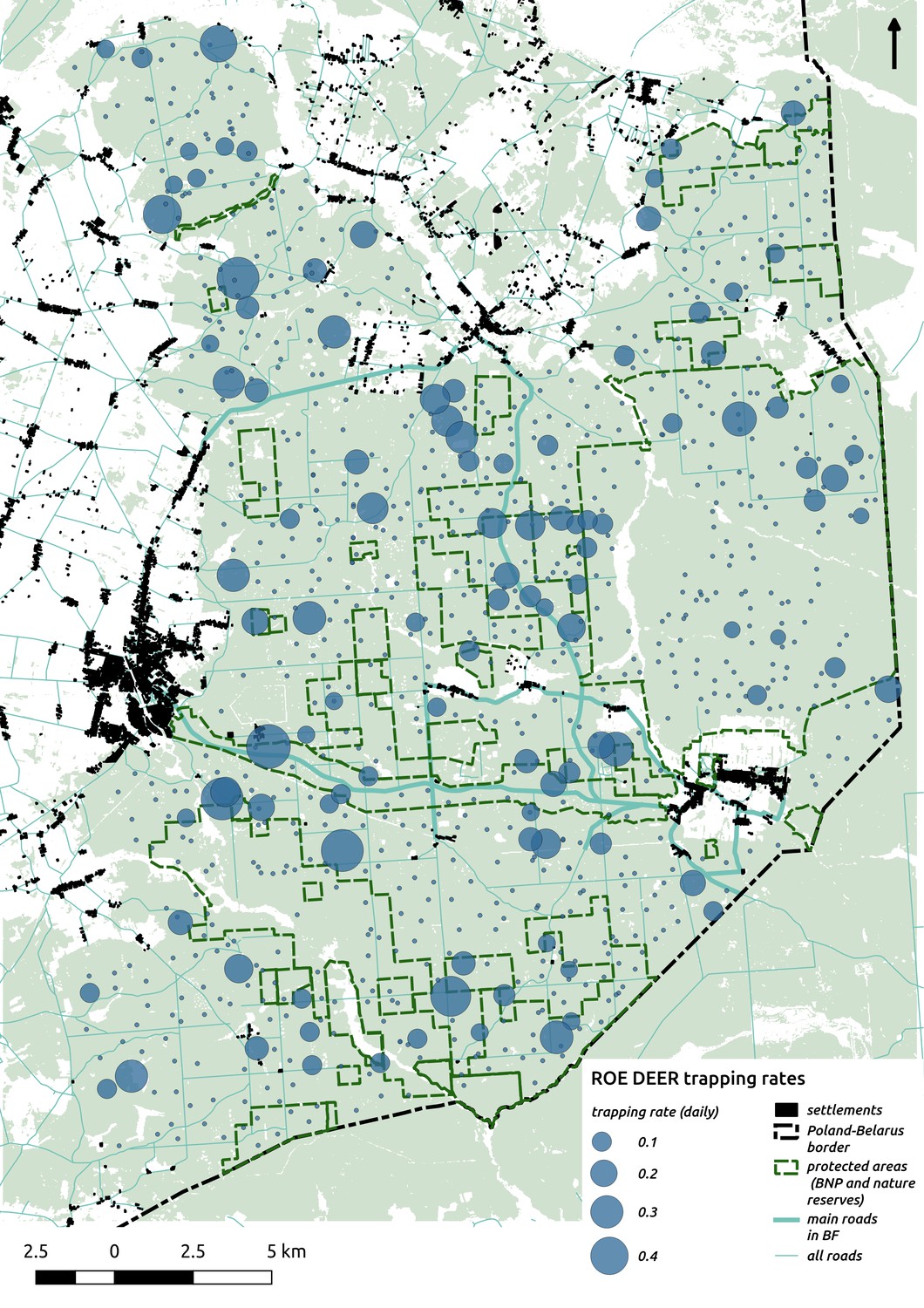
Bubble plot presenting raw camera trapping data for roe deer collected during the ungulate survey.
Each bubble is a camera trap location and its size is proportional to the daily trapping rate (i.e. no. of individuals observed/no. of days).
Appendix 1—figure 10
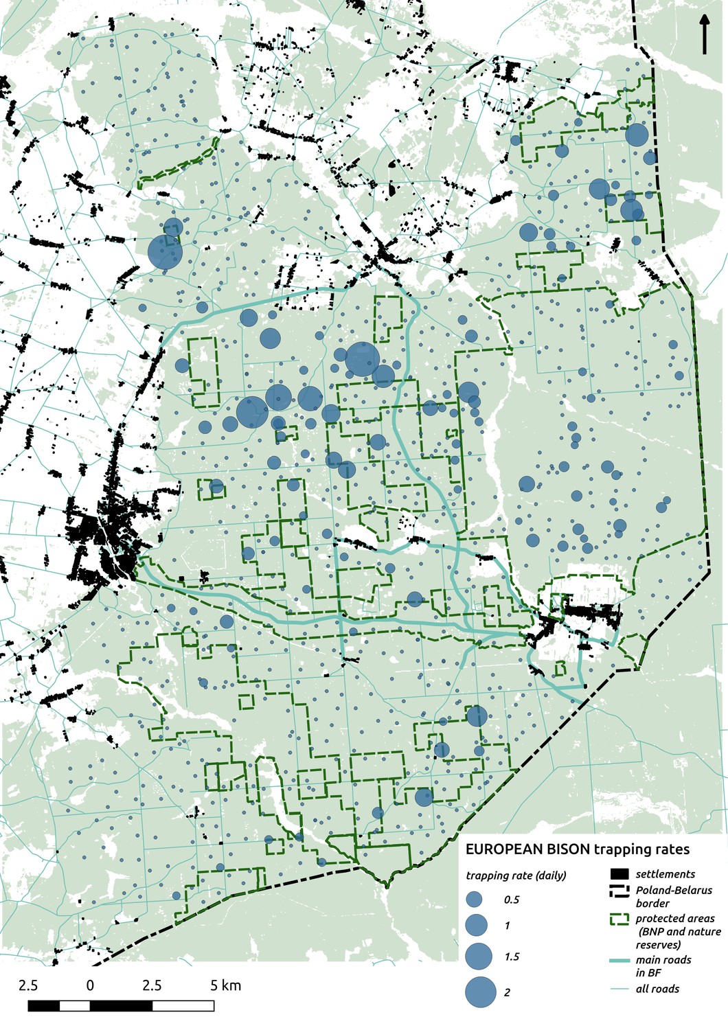
Bubble plot presenting raw camera trapping data for bison collected during the ungulate survey.
Each bubble is a camera trap location and its size is proportional to the daily trapping rate (i.e. no. of individuals observed/no. of days).
Appendix 1—figure 11
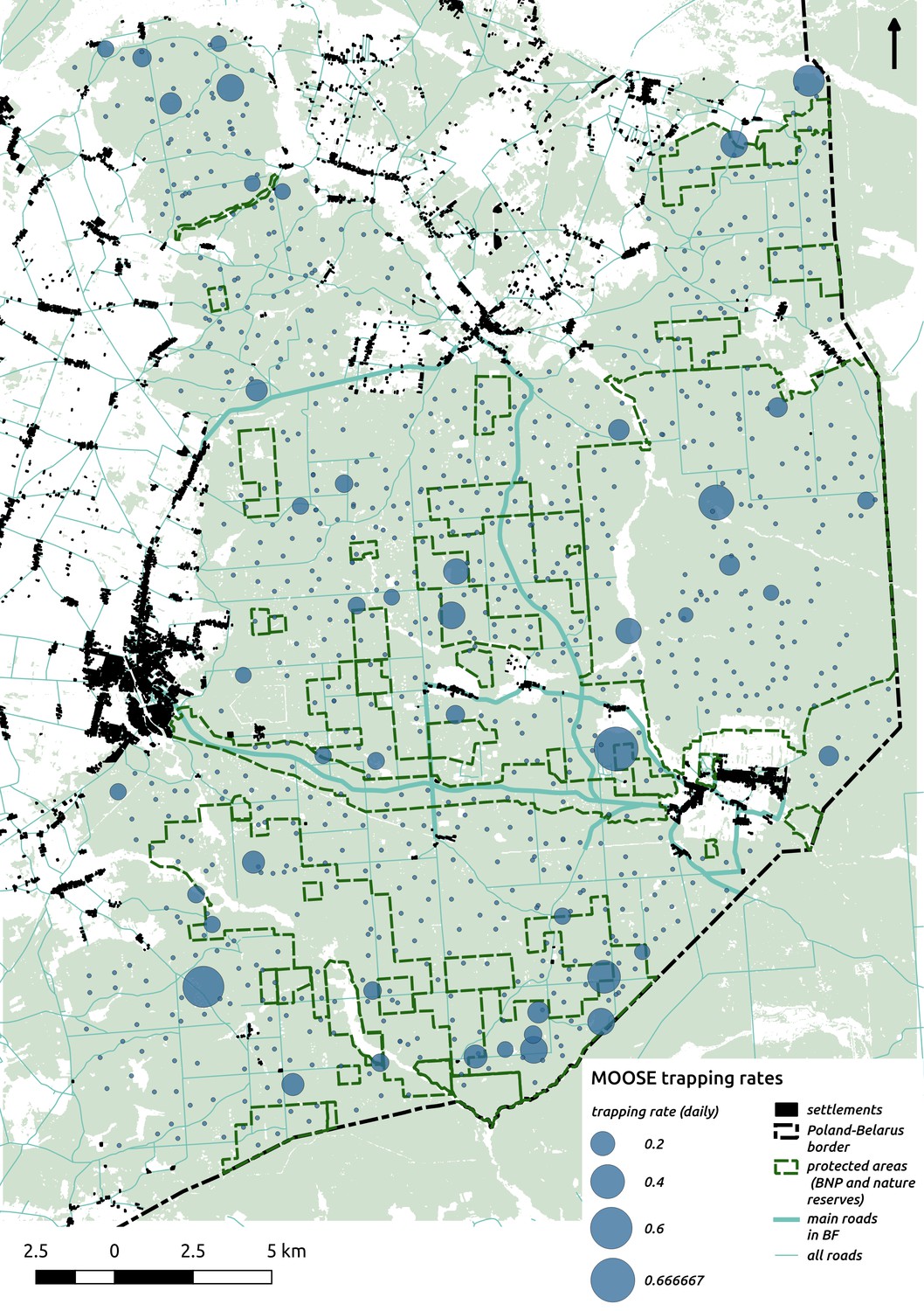
Bubble plot presenting raw camera trapping data for moose collected during the ungulate survey.
Each bubble is a camera trap location and its size is proportional to the daily trapping rate (i.e. no. of individuals observed/no. of days).
Appendix 1—figure 12
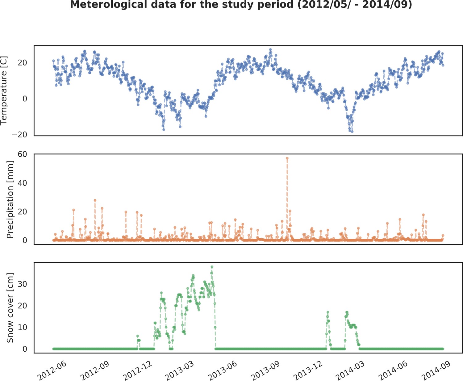
Basic meteorological data for the study period (05/2012 – 09/2014): 1) averaged daily temperature [C], 2) precipitation [mm] and 3) snow cover [cm].
https://doi.org/10.7554/eLife.44937.034
Appendix 1—figure 13

Distribution of camera trap locations grouped by quality of view in front of a camera and different UNESCO zones in Białowieża Forest (1: Strict Reserve of BNP, 2: BNP and nature reserves, 3: valuable unprotected forest stands, 4: managed forest stands).
Each camera location was manually tagged with a 4-level categorical label (‘Exclude’, ‘Acceptable’, ‘Good’, ‘Perfect’) describing the quality of view in front of the camera. Locations labeled with the ‘Exclude’ were not included in further analysis and are not shown on this figure.
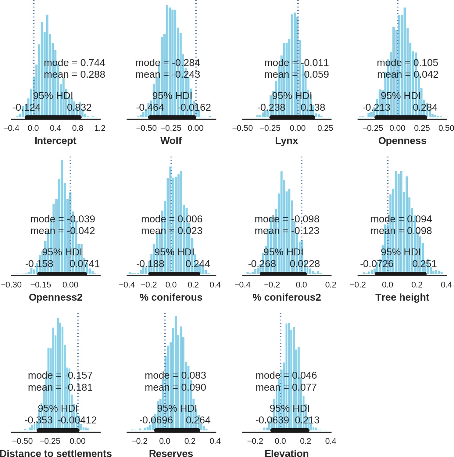
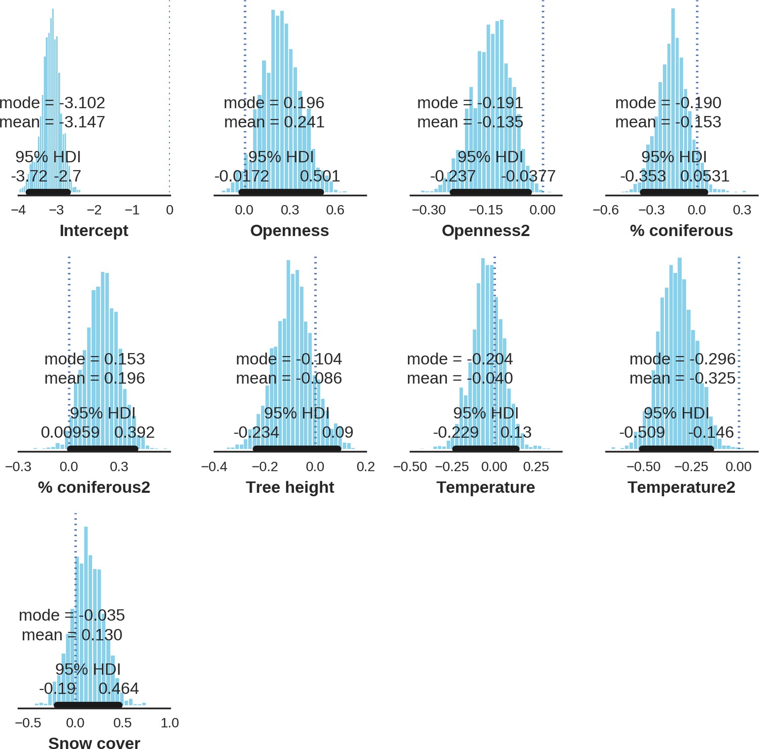
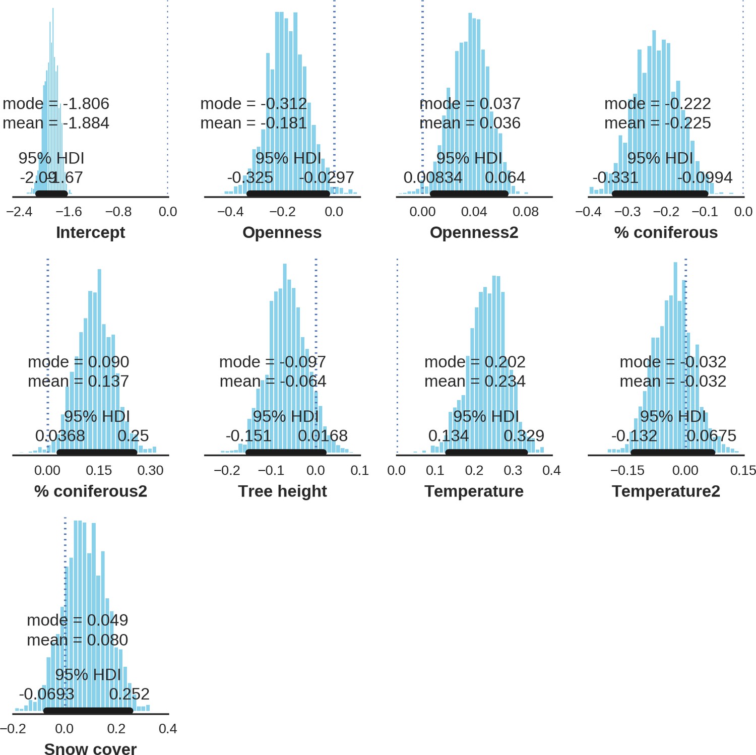
Appendix 1—figure 14
Red deer female – landscape use; the posterior distributions of all parameters.
https://doi.org/10.7554/eLife.44937.036
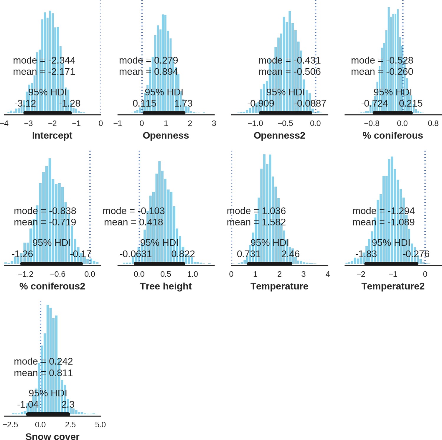
Appendix 1—figure 15
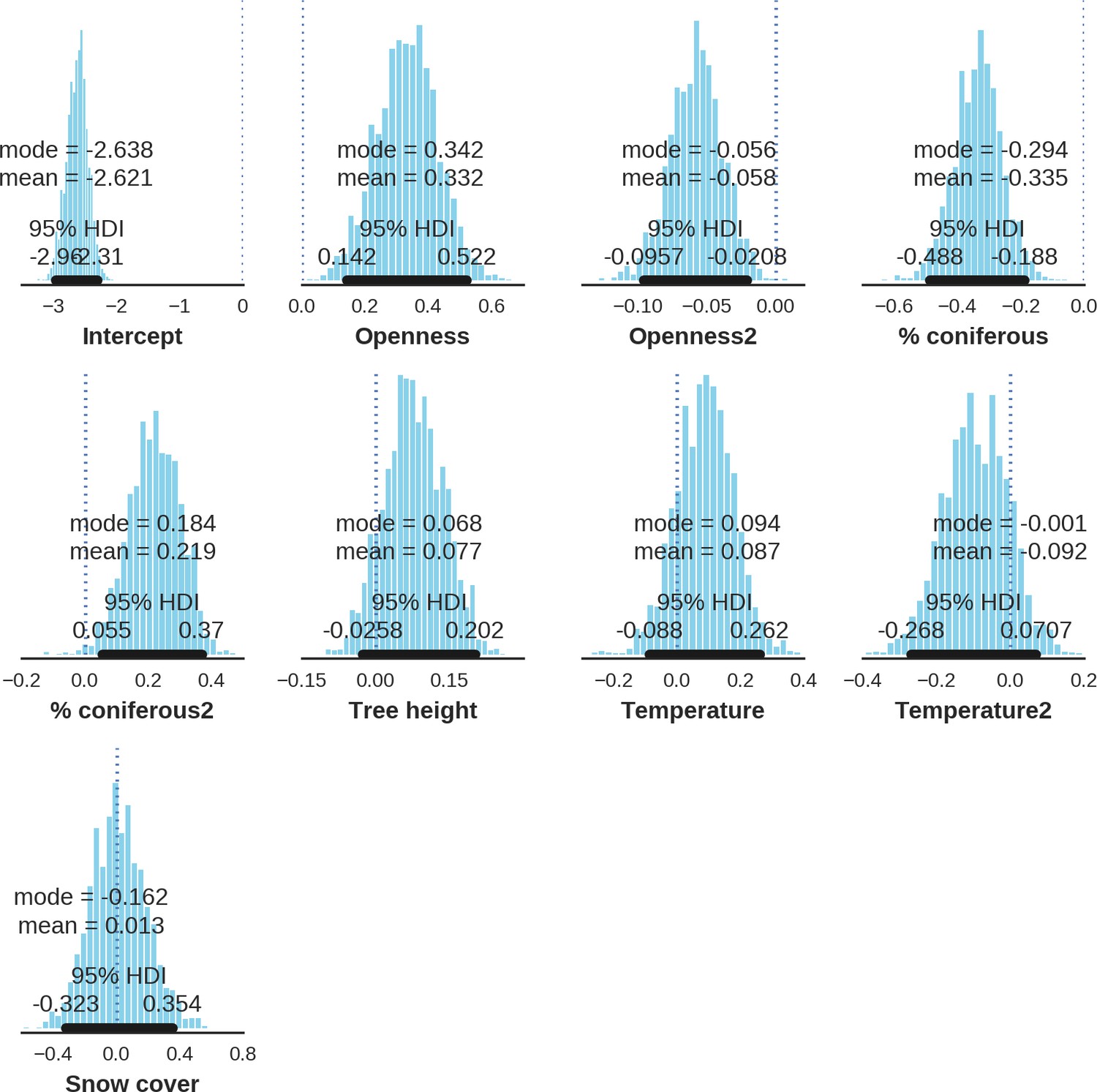
Red deer female – detection rate; the posterior distributions of all parameters.
https://doi.org/10.7554/eLife.44937.037
Appendix 1—figure 16
Red deer male – landscape use; the posterior distributions of all parameters.
https://doi.org/10.7554/eLife.44937.038
Appendix 1—figure 17
Red deer male – detection rate; the posterior distributions of all parameters.
https://doi.org/10.7554/eLife.44937.039
Appendix 1—figure 18
Roe deer – landscape use; the posterior distributions of all parameters.
https://doi.org/10.7554/eLife.44937.040
Appendix 1—figure 19
Roe deer – detection rate; the posterior distributions of all parameters.
https://doi.org/10.7554/eLife.44937.041
Appendix 1—figure 20
Wild boar – landscape use; the posterior distributions of all parameters.
https://doi.org/10.7554/eLife.44937.042
Appendix 1—figure 21
Wild boar – detection rate; the posterior distributions of all parameters.
https://doi.org/10.7554/eLife.44937.043
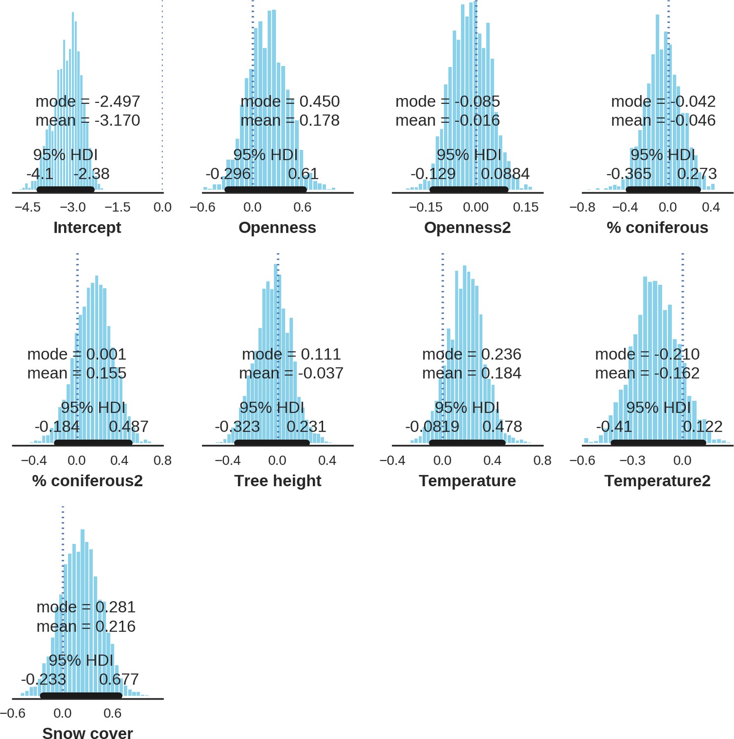
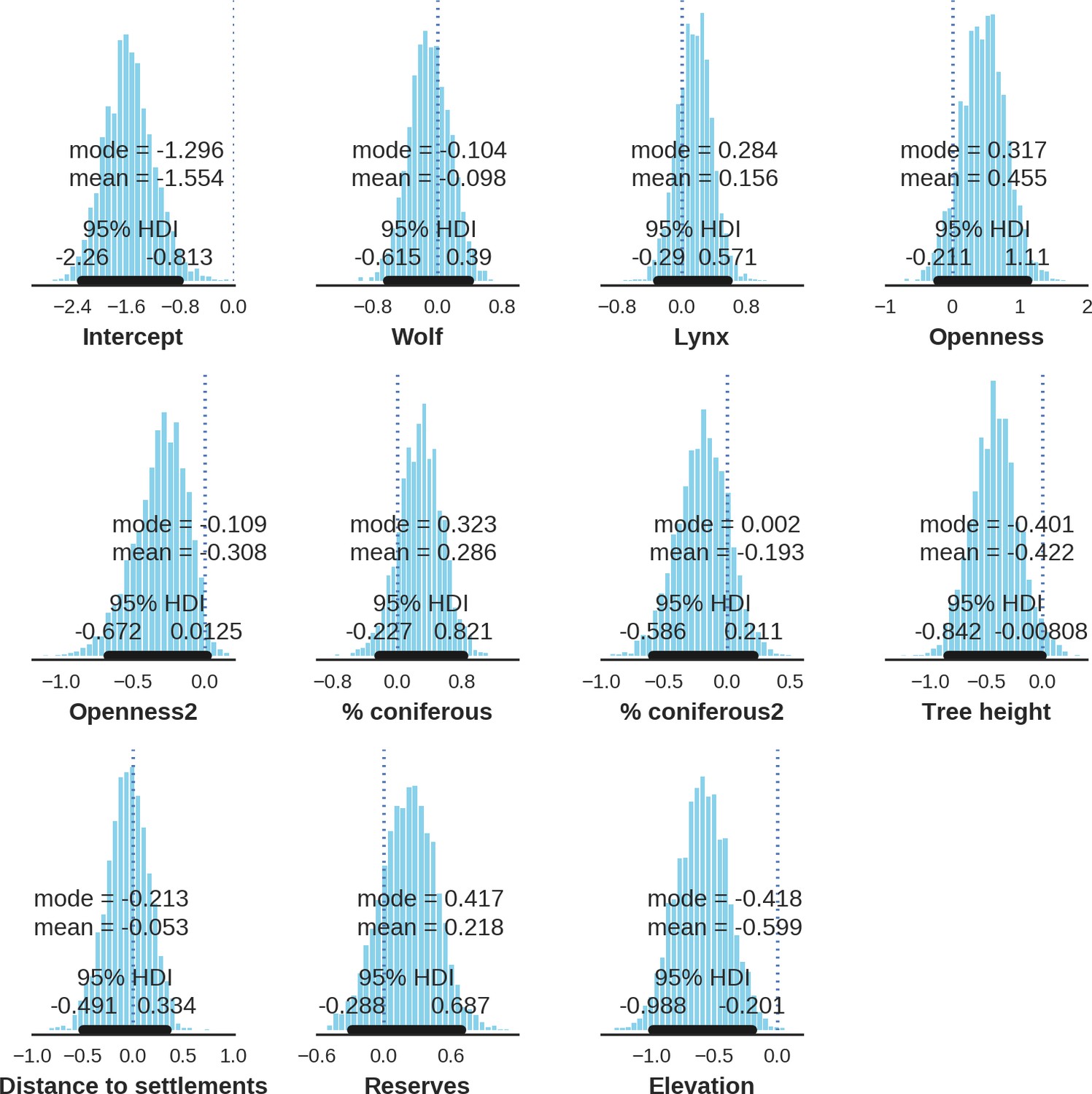
Appendix 1—figure 22
European bison – landscape use; the posterior distributions of all parameters.
https://doi.org/10.7554/eLife.44937.044
Appendix 1—figure 23
European bison – detection rate; the posterior distributions of all parameters.
https://doi.org/10.7554/eLife.44937.045
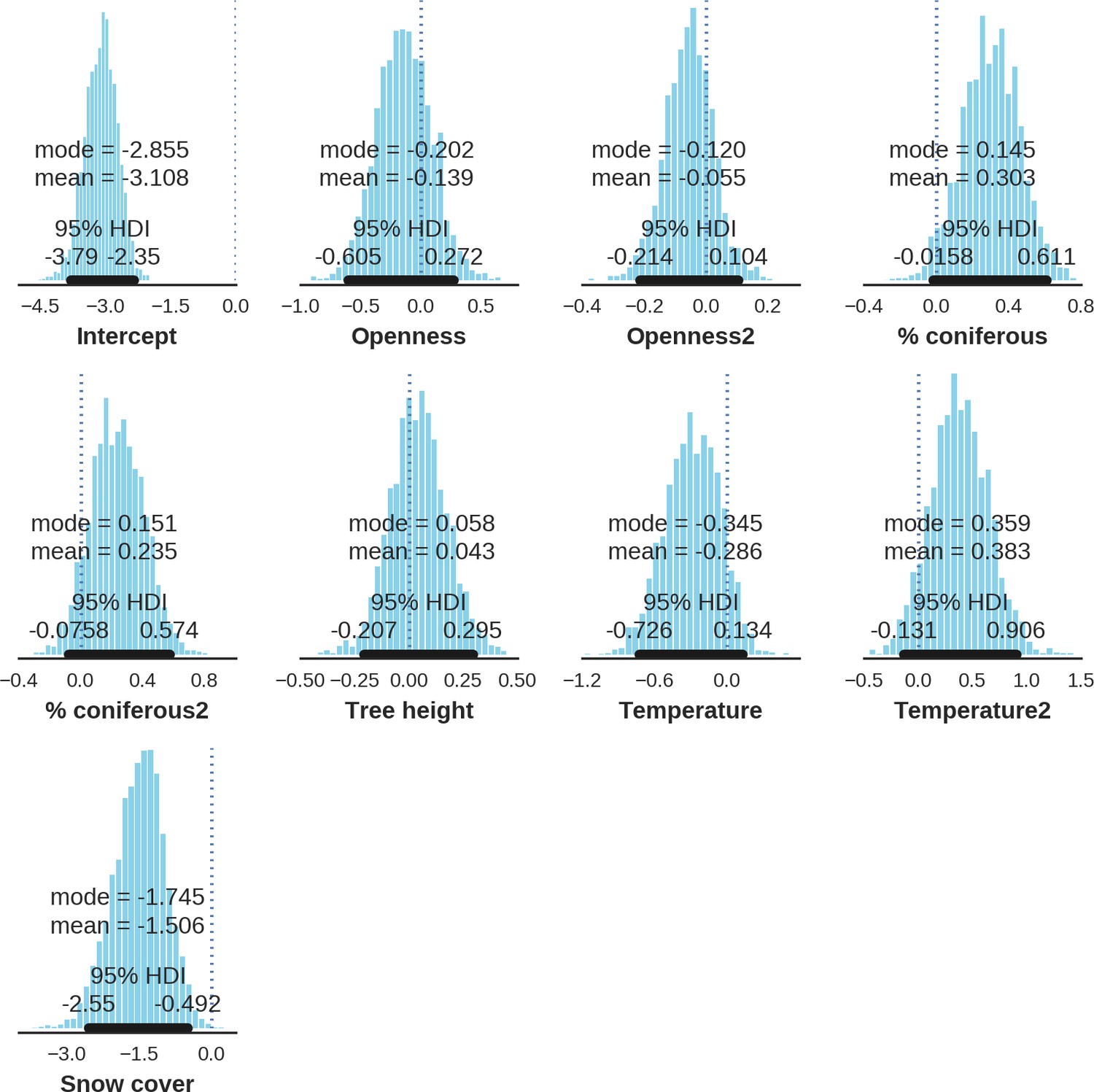
Appendix 1—figure 24
Moose – landscape use; the posterior distributions of all parameters.
https://doi.org/10.7554/eLife.44937.046
Appendix 1—figure 25
Moose – detection rate; the posterior distributions of all parameters.
https://doi.org/10.7554/eLife.44937.047
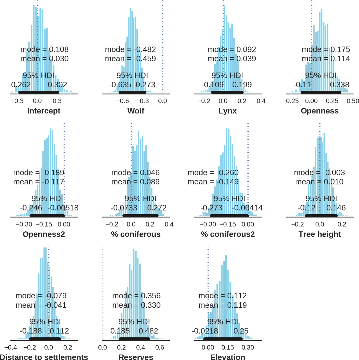
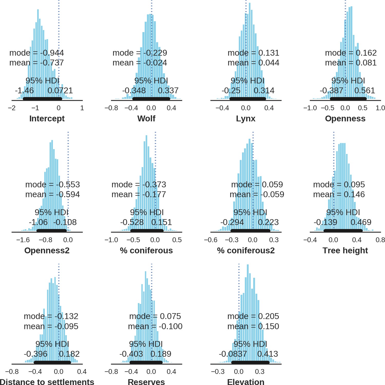
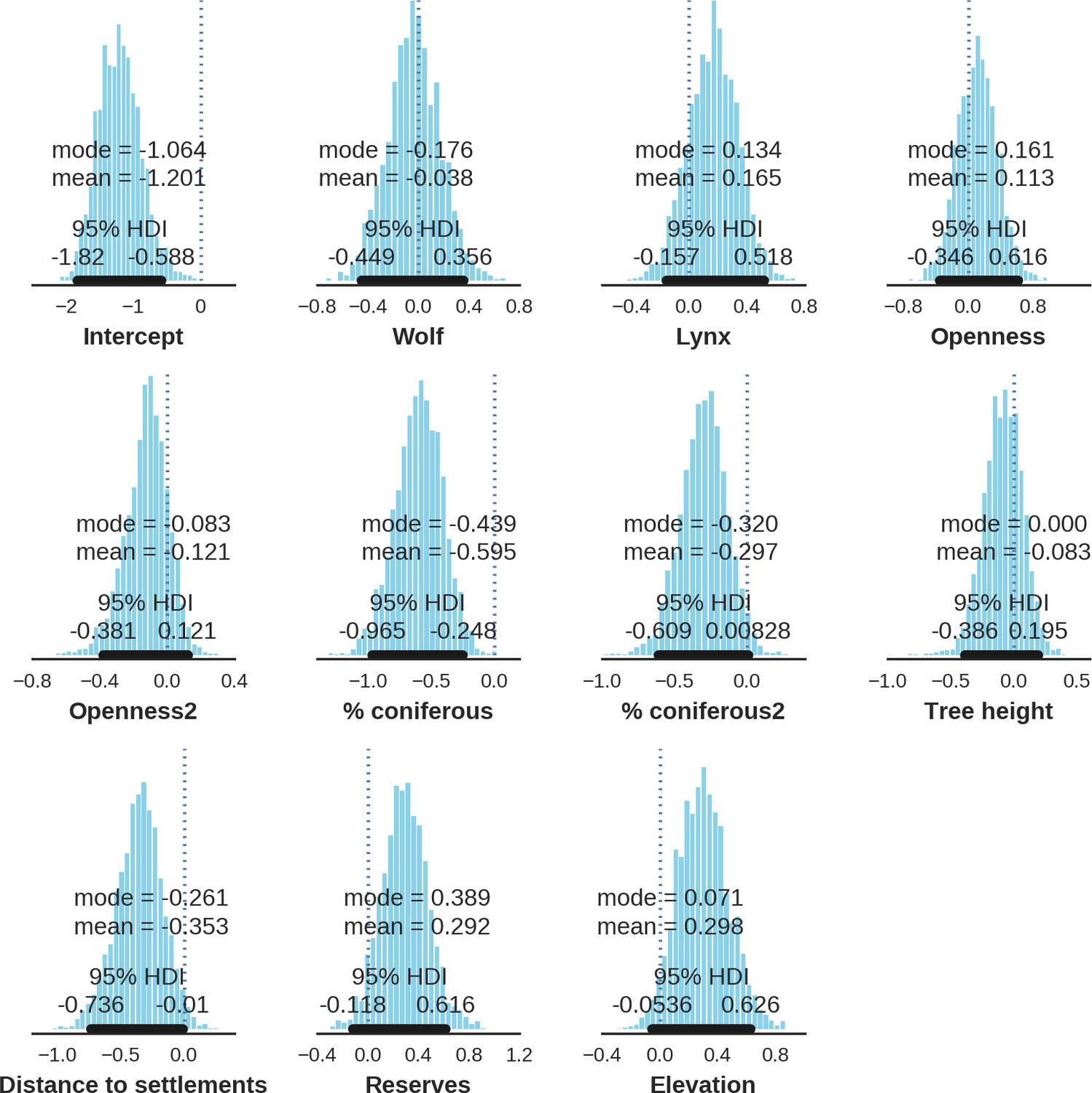
Appendix 1—figure 26
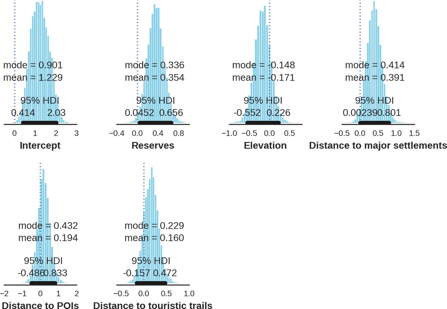
Wolf – landscape use; the posterior distributions of all parameters.
https://doi.org/10.7554/eLife.44937.048
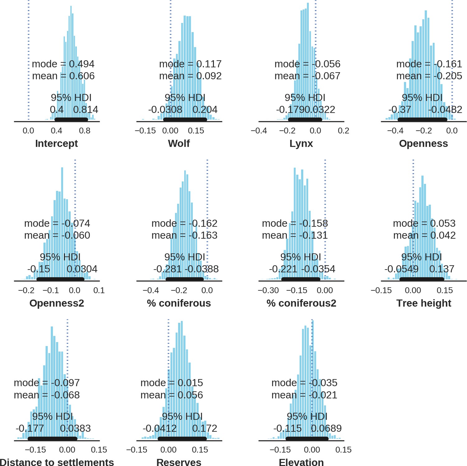
Appendix 1—figure 27
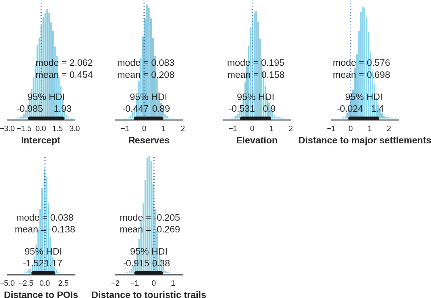
Eurasian lynx – landscape use; the posterior distributions of all parameters.
https://doi.org/10.7554/eLife.44937.049
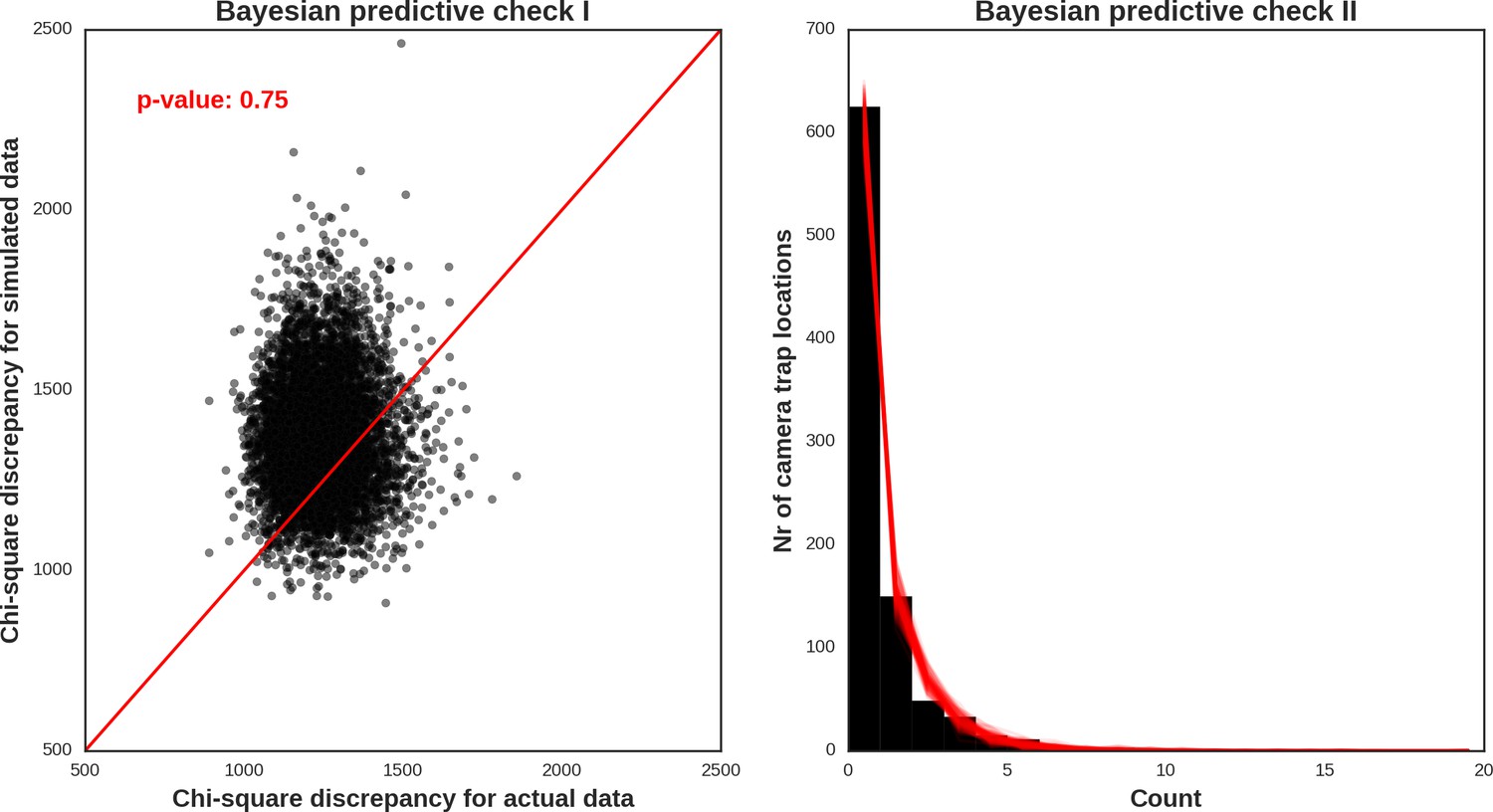
Appendix 1—figure 28
Red deer female – model diagnostic plots.
https://doi.org/10.7554/eLife.44937.050
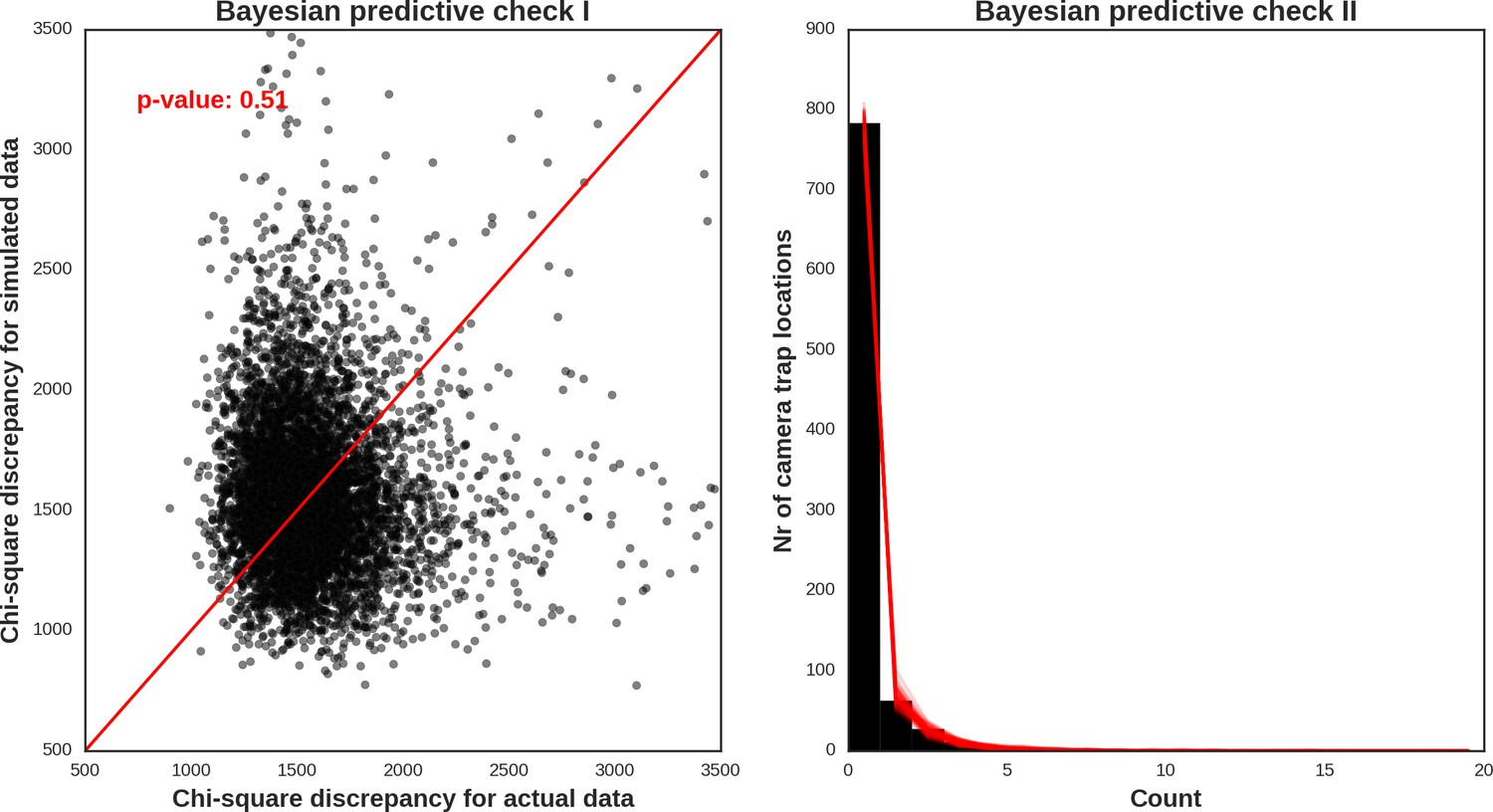
Appendix 1—figure 29
Red deer male – model diagnostic plots.
https://doi.org/10.7554/eLife.44937.051
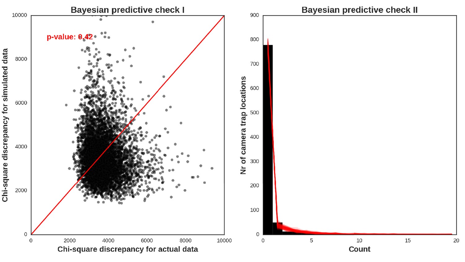
Appendix 1—figure 30
Roe deer – model diagnostic plots.
https://doi.org/10.7554/eLife.44937.052
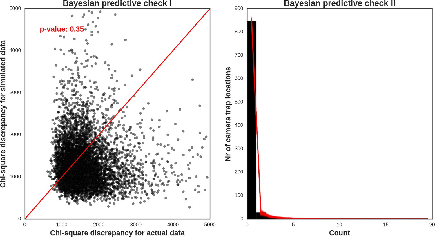
Appendix 1—figure 31

Wild boar – model diagnostic plots.
https://doi.org/10.7554/eLife.44937.053
Appendix 1—figure 32
European bison – model diagnostic plots.
https://doi.org/10.7554/eLife.44937.054
Appendix 1—figure 33
Moose – model diagnostic plots.
https://doi.org/10.7554/eLife.44937.055
Appendix 1—figure 34

Wolf – model diagnostic plots.
https://doi.org/10.7554/eLife.44937.056
Appendix 1—figure 35
Eurasian lynx – model diagnostic plots.
https://doi.org/10.7554/eLife.44937.057
Appendix 1—figure 36
Estimated effects of the covariates from the model for all ungulate species using only a subset of camera trap data covering a three month period (August - October) closely matching the period of the carnivore survey.
The covariates explain the spatial variation in the parameter , which is the expected number of individuals using a given landscape grid cell (25 ha pixel) during the sampling period (i.e. the relative density; see the general and formal description of the model in the Materials and methods section).
Appendix 1—figure 37

The spatial predictions for the parameter , which is the expected number of individuals using a given landscape grid cell (25 ha pixel) during the sampling period (see the general and formal description of the model in the Materials and methods section).
The predictions are based on the model for all ungulate species using only a subset of the camera trap data covering a three month period (August - October) closely matching the period of the carnivore survey.
Tables
Appendix 1—table 1
Summary of the two camera trapping surveys conducted during the study period.
Days – the total number of trapping days (effort), Counts – the total number of individuals recorded during independent visits (events), Trate – trapping rate. Notice the dramatic differences in the trapping rates of the carnivores between the two types of surveys. Counts of red deer female (973) and red deer male (547) do not sum to the total count (2025) as there were 505 records of individuals of undefined gender.
| Species | Days | Counts | Trate (daily) | Trate sd | Trate max |
|---|---|---|---|---|---|
| Ungulates survey (05.2012–05.2014) | |||||
| Wild Boar | 9813 | 4818 | 0.49507 | 0.87881 | 10.16667 |
| Red Deer | 9813 | 2025 | 0.20255 | 0.36340 | 3.90909 |
| Red Deer Female | 9813 | 973 | 0.09648 | 0.20391 | 2.00000 |
| Red Deer Male | 9813 | 547 | 0.05544 | 0.12867 | 1.25000 |
| European Bison | 9813 | 440 | 0.04522 | 0.23212 | 4.50000 |
| Roe Deer | 9813 | 194 | 0.02043 | 0.06611 | 0.54545 |
| Eurasian Elk | 9813 | 82 | 0.00866 | 0.04714 | 0.66667 |
| Wolf | 9813 | 51 | 0.00541 | 0.02960 | 0.36364 |
| Eurasian Lynx | 9813 | 3 | 0.00027 | 0.00458 | 0.08333 |
| Carnivores survey (09–10.2015) | |||||
| Wolf | 3093 | 471 | 0.19129 | 0.49534 | 6.00000 |
| Eurasian Lynx | 3093 | 35 | 0.01268 | 0.04997 | 0.33333 |
Appendix 1—table 2
Matrix of the foraging-related traits used for the estimation of the functional diversity index (FDis) of the entire ungulate community: body mass (based on Jedrzejewska et al., 1994) and Borowik et al., 2016), diet type (based on Hofmann, 1989); B: browsers-concentrate selectors, BG: browsers/grazers-intermediate types, G: grazers-grass roughage eaters, O: omnivores) and gut type (R: ruminants, NR: non-ruminants).
https://doi.org/10.7554/eLife.44937.022| Roe deer | Wild boar | Red deer female | Red deer male | Moose | European bison | |
|---|---|---|---|---|---|---|
| Body mass | 20 | 80 | 90 | 150 | 200 | 400 |
| Diet type | B | O | BG | BG | B | G |
| Gut type | R | NR | R | R | R | R |
Additional files
-
Source data 1
Source data tables and Python code of the analysis.
- https://doi.org/10.7554/eLife.44937.017
-
Supplementary file 1
MCMC trace plots.
- https://doi.org/10.7554/eLife.44937.018
-
Transparent reporting form
- https://doi.org/10.7554/eLife.44937.019
Download links
A two-part list of links to download the article, or parts of the article, in various formats.
Downloads (link to download the article as PDF)
Open citations (links to open the citations from this article in various online reference manager services)
Cite this article (links to download the citations from this article in formats compatible with various reference manager tools)
Linking spatial patterns of terrestrial herbivore community structure to trophic interactions
eLife 8:e44937.
https://doi.org/10.7554/eLife.44937


