The dynamic conformational landscape of the protein methyltransferase SETD8
- Memorial Sloan Kettering Cancer Center, United States
- Shanghai Institute of Materia Medica, Chinese Academy of Sciences, China
- Icahn School of Medicine at Mount Sinai, United States
- University of Toronto, Canada
- University of Georgia, United States
- Science Center Drive, United States
- University of Chinese Academy of Sciences, China
- Weill Cornell Medical College of Cornell University, United States
Figures
Figure 1 with 5 supplements
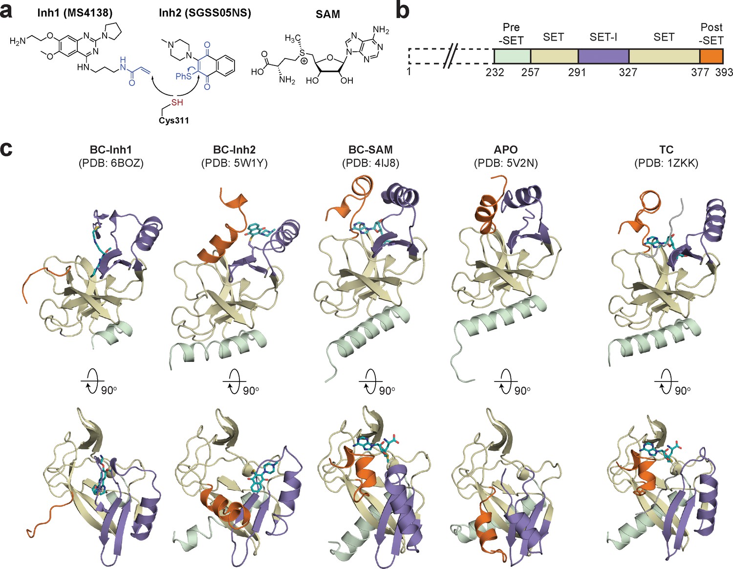
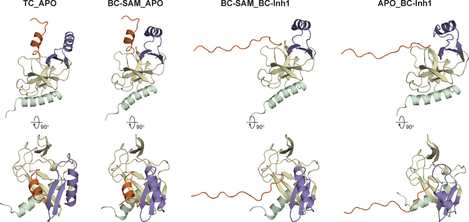
Diverse SETD8 conformations captured in altered ligand-binding states.
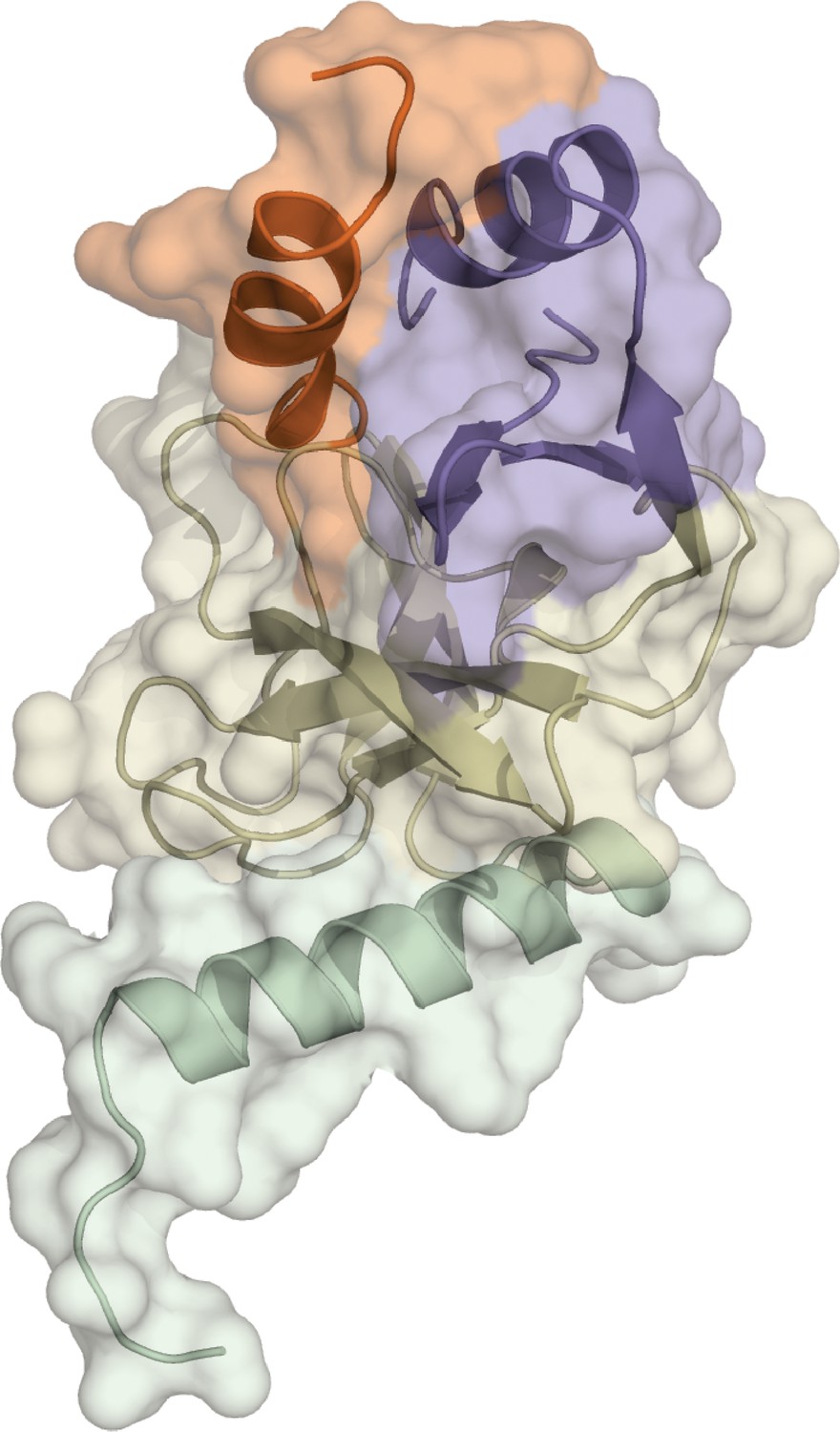
(a) Structures of SETD8 ligands involved in this work. Two covalent inhibitors targeting Cys311 (MS4138 as Inh1 and SGSS05NS as Inh2) and the cofactor SAM were used as ligands to trap neo-conformations of SETD8. (b) Domain topology of SETD8 (Uniprot: Q9NQR1-1). Four functional motifs at SETD8’s catalytic domain are colored: pre-SET (light green), SET (dark yellow), SET-I (purple), and post-SET (orange). (c) Cartoon representations of four neo-structures of SETD8 (BC-Inh1, BC-Inh2, BC-SAM, and APO) and a structure of a SETD8-SAH-H4 ternary complex (TC). These structures are shown in two orthogonal views with ligands, pre-SET, SET, SET-I, and post-SET colored in cyan, light green, dark yellow, purple, and orange, respectively.
Figure 1—figure supplement 1
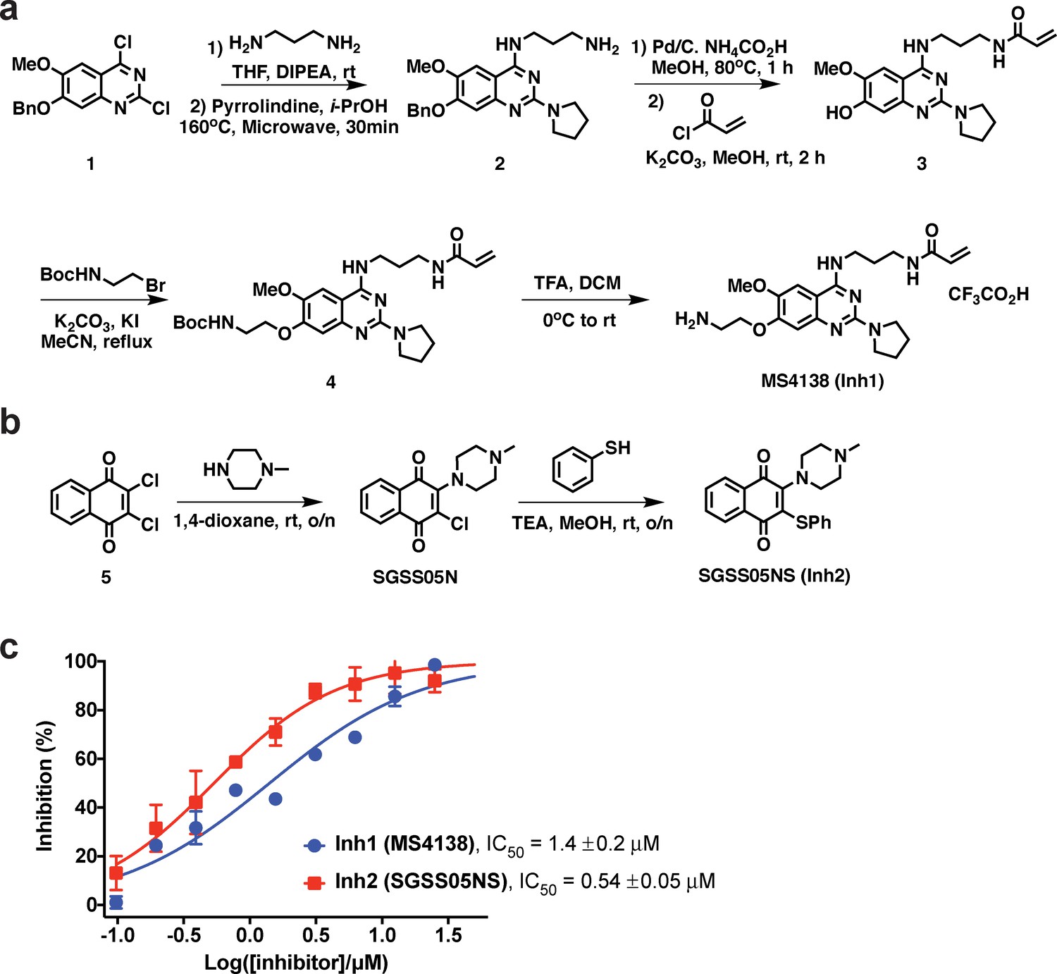
Synthesis and characterization of two covalent inhibitors targeting SETD8.
(a) Synthesis of MS4138 (Inh1). (b) Synthesis of SGSS05NS (Inh2). (c) Inhibition and IC50 curves of wild-type SETD8 with two covalent inhibitors (Inh1/2) determined by in vitro radiometric assay. Data are best fitting values ± s.e. from Prism7.
Figure 1—figure supplement 2
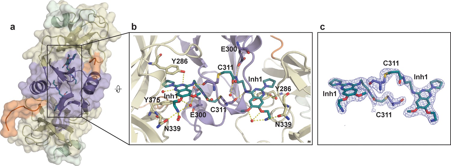
Crystal structure of SETD8 in complex with Inh1 (BC-Inh1).
(a) the overall structure of the homodimer of SETD8-Inh1 complex. (b) details of protein-ligand interactions. (Inh1), which is covalently conjugated with one monomer, is inserted into the substrate binding pocket of the other monomer (right). Key interactions of Inh1) with nearby residues and water molecules are shown with yellow dashed lines. (c) omit map of electron density of the ligand (Inh1) and conjugated Cys (C311). The color code of motifs is the same as used in Figure 1.
Figure 1—figure supplement 3
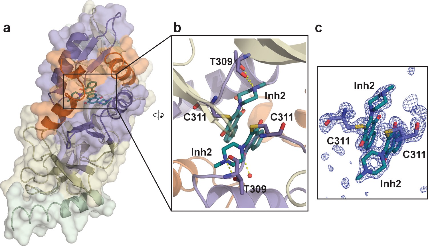
Crystal structure of SETD8 in complex with Inh2 (BC-Inh2).
(a) the overall structure of the homodimer of SETD8-Inh2 complex. (b) details of protein-ligand interactions. The two Inh2 molecules, which are covalently conjugated to the SETD8 homodimer, interact via pi-pi stacking (right). Key interactions of Inh2 with nearby residues and water molecules are shown as yellow dashed lines. (c) Omit mFo-DFc density for the ligand (Inh2) and conjugated Cys (C311). Map coefficients were calculated with PHENIX and contoured at level 3 with PyMOL. The color code of motifs is the same as used in Figure 1.
Figure 1—figure supplement 4
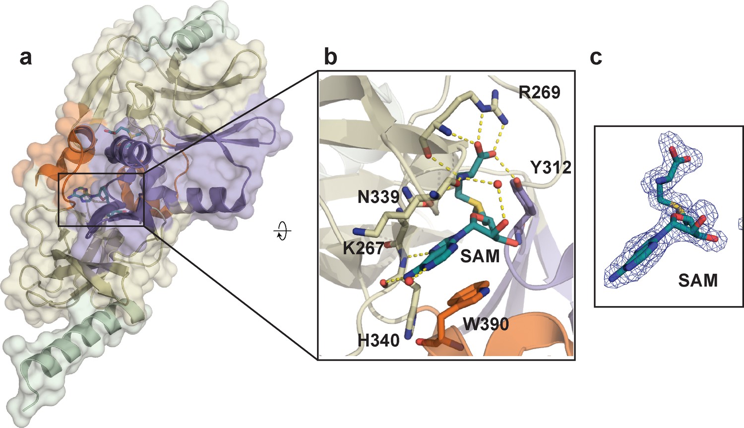
Crystal structure of SETD8 in complex with the cofactor SAM (BC-SAM).
(a) the overall structure of the homodimer of SETD8-SAM complex. (b) details of protein-ligand interactions. Key interactions of SAM with nearby residues and water molecules are shown as yellow dashed lines (right). (c) Omit mFo-DFc density for SAM. Map coefficients were calculated with PHENIX and contoured at level three with PyMOL. The color code of motifs is the same as used in Figure 1.
Figure 1—figure supplement 5
Crystal structure of apo SETD8 (APO).
The crystal structure of apo SETD8 was determined as a monomer. The color code of motifs is the same as used in Figure 1.
Figure 2
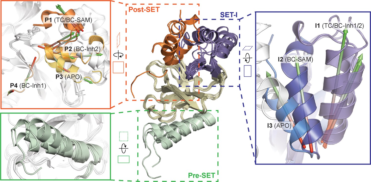
Superposition of five crystal structures highlighted with detailed views of post-SET, SET-I, and pre-SET motifs.
The five X-ray structures reveal four distinct conformational states of the post-SET motif (P1-4) and three distinct conformational states of the SET-I motif (I1-3).
Figure 3 with 2 supplements
Construction of conformational landscapes of apo- and SAM-bound SETD8 through diversely seeded, parallel molecular dynamics simulations and Markov state models.
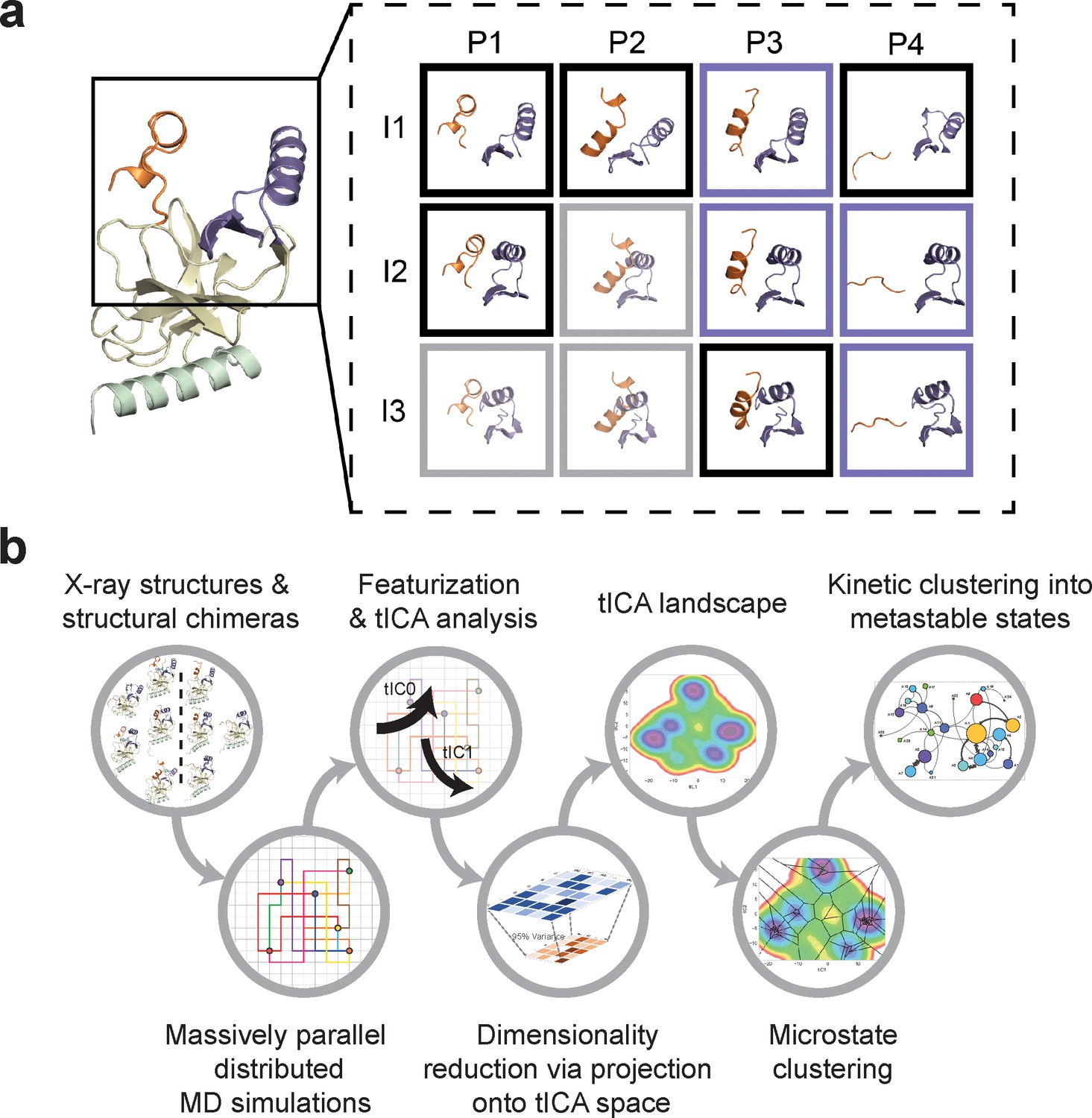
(a) Combinatorial construction of putative structural domain chimeras using crystallographically-derived post-SET and SET-I conformations. Each conformer is boxed and color-coded with black for five X-ray-derived structures, blue for four putative structural chimeras included as seed structures for MD simulations, and gray for three structural chimeras excluded from MD simulations because of obvious steric clashes. (b) Schematic workflow to construct dynamic conformational landscapes via MSM. The five X-ray structures and the four structural chimeras were used to seed parallel MD simulations on Folding@home (see Materials and method). Markov state models were constructed from these MD simulation results to reveal the conformational landscape.
Figure 3—figure supplement 1

Workflow of MD simulations and MSM analysis.
On the basis of X-ray structures of SETD8, we prepared nine seed conformations of apo-SETD8 simulations and two seed conformations of SAM-bound SETD8 simulations, from which 5020 and 1000 molecular dynamics (MD) trajectories were initiated on Folding@home, respectively. The data of apo-SETD8 were used to search optimal hyperparameters for Markov state models (MSMs) via variational scoring combined with cross-validation. Dihedral features (phi, psi, chi1), tICA lag time of 5 ns, tICA commute mapping and 100 microstates were selected as the best set of hyperparameters for MSMs with the lag time of 50 ns. Models were fitted with the data of apo-SETD8 and the data of SAM-bound SETD8 were transformed in the same degrees of freedom as those of apo-SETD8. Hidden Markov models (HMMs) of apo- and SAM-bound SETD8 were then generated and used for structural annotation of all conformations.
Figure 3—figure supplement 2
Cartoon representations of the four structural chimeras.
Conformations of structural chimeras (prior to simulation) are shown. Orientations and the color code of motifs are the same as used in Figure 1.
Figure 4
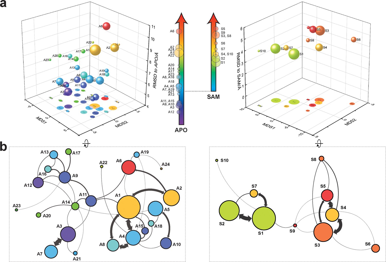
Markov state models and conformational landscapes of apo- and SAM-bound SETD8.
Kinetically metastable conformations (macrostates) obtained from kinetically coupled microstates via Hidden Markov Model (HMM) analysis. The revealed dynamic conformational landscapes consist of 24 macrostates for apo-SETD8 (left panel) and 10 macrostates for SAM-bound SETD8 (right panel). (a) Kinetic and structural separation of macrostates in a 3D scatterplot. The MDS1/MDS2 axes are the two top vectors used in multidimensional scaling (MDS), a dimensionality reduction method, for separation of macrostates via log-inverse flux kinetic embedding (see Materials and methods). The Z axis reports root-mean-square deviations (RMSDs) of each macrostate to APO (left) or BC-SAM (right). The relative population of each macrostate of apo- or SAM-bound SETD8 ensembles is proportional to the volume of each representative sphere. (b) Cartoon depiction of macrostates in a 2D scatterplot. The diameter of the corresponding circle in the 2D scatterplot is proportional to the diameter of the respective sphere in the 3D scatterplot above. Equilibrium kinetic fluxes larger than 7.14 × 10² s−1 for apo- and 1.39 × 10³ s−1 for SAM-bound SETD8 are shown for interconversion kinetics with thickness of the connections proportional to fluxes between two macrostates.
Figure 5 with 2 supplements
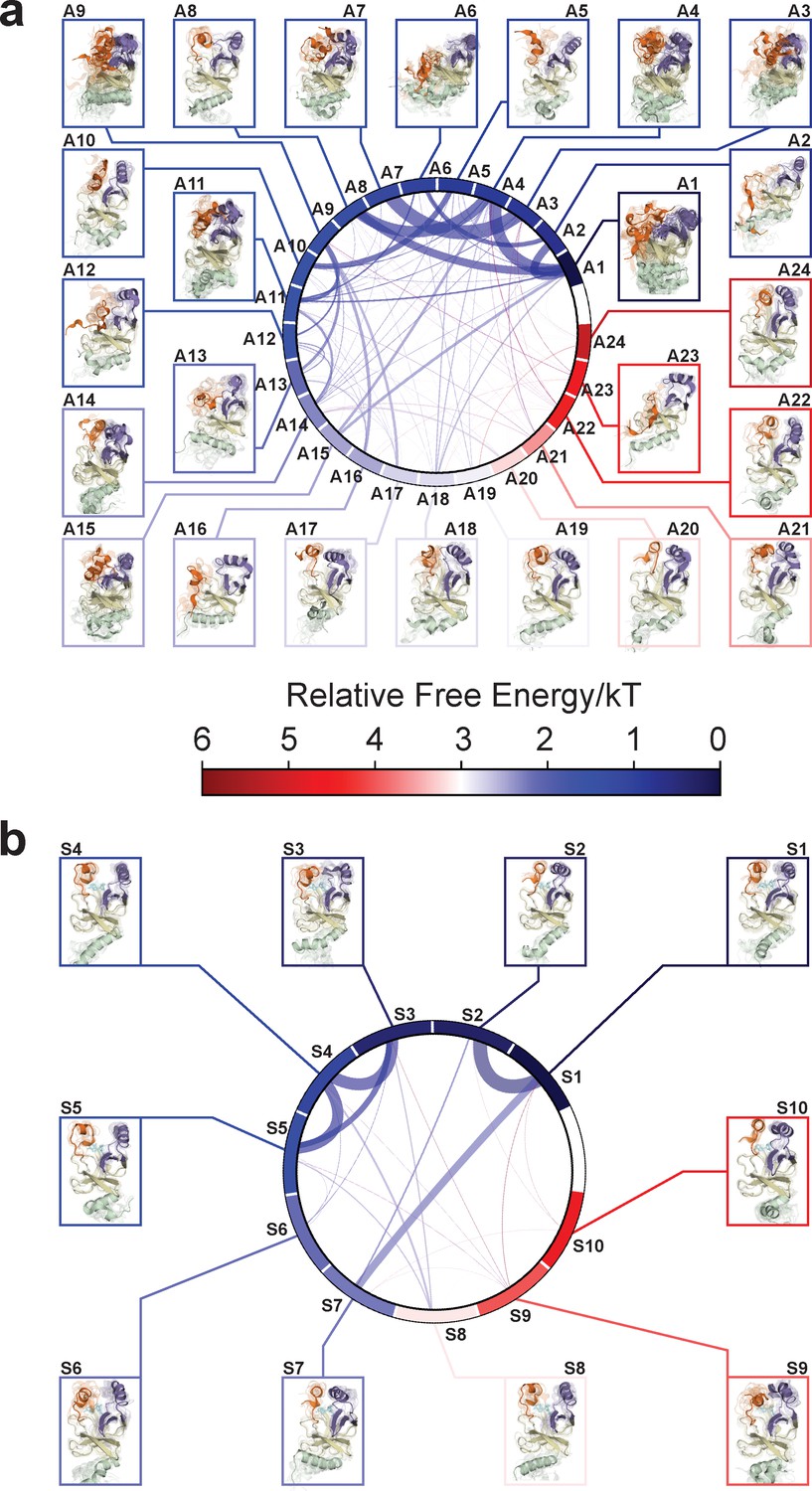
Chord diagrams and representative conformers of macrostates.
The colors represent the free energy of each macrostate relative to the lowest free energy macrostate. The equilibrium flux between two macrostates is proportional to thickness of connecting arcs.
Figure 5—figure supplement 1
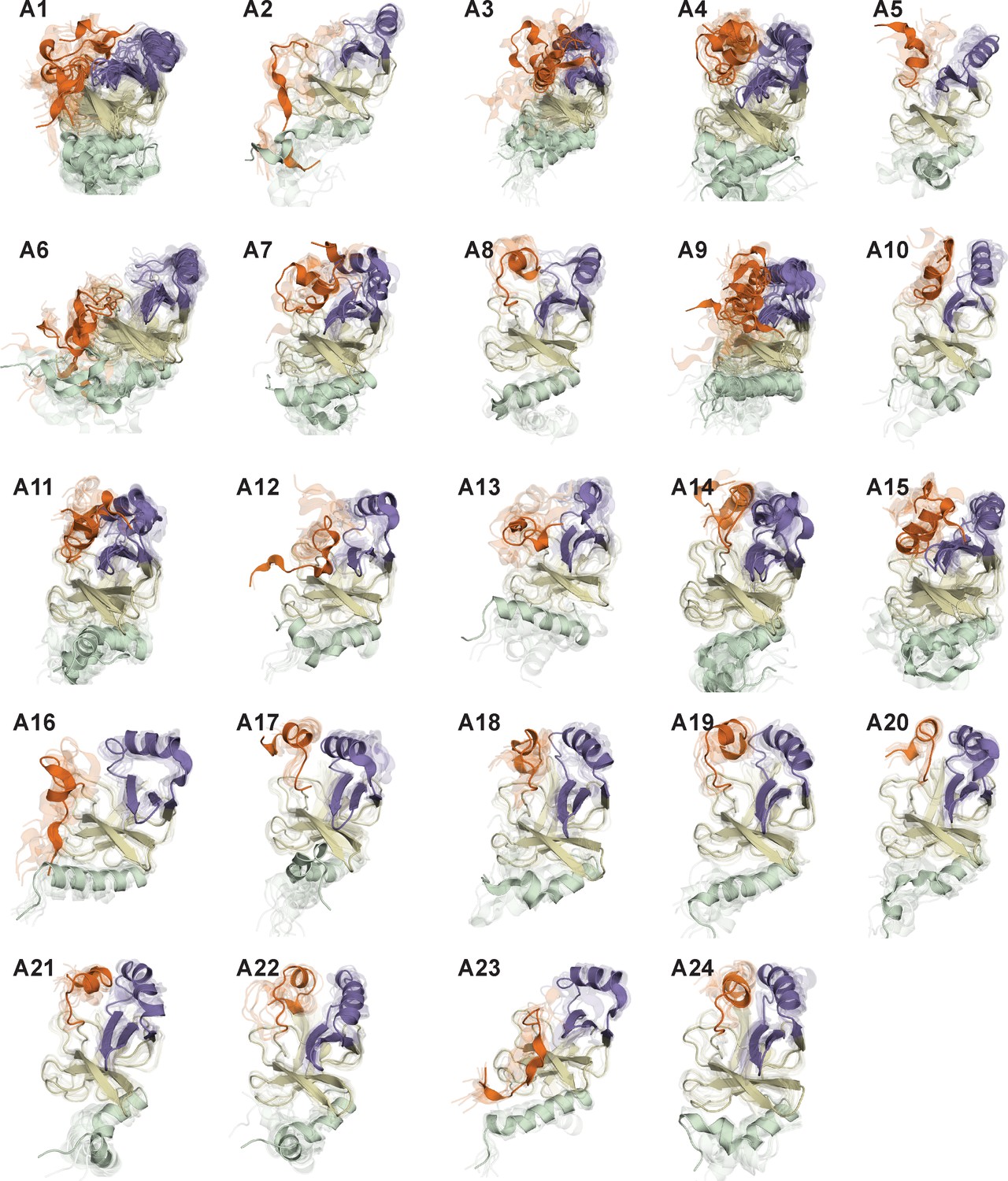
Representative conformations of macrostates in the conformational landscape of apo-SETD8.
For macrostates with high structural homogeneity (A2, A5, A8, A10, A12, A13, A16 ~24), 10 frames closest to the center of the microstate with the largest observation probability are presented. For macrostates with high structural diversity (A1, A3, A4, A6, A7, A9, A11, A12, A14), multiple microstates with the sum of observation probabilities > 0.5 are selected, and 10 frames closest to the center of each microstate are presented together.
Figure 5—figure supplement 2
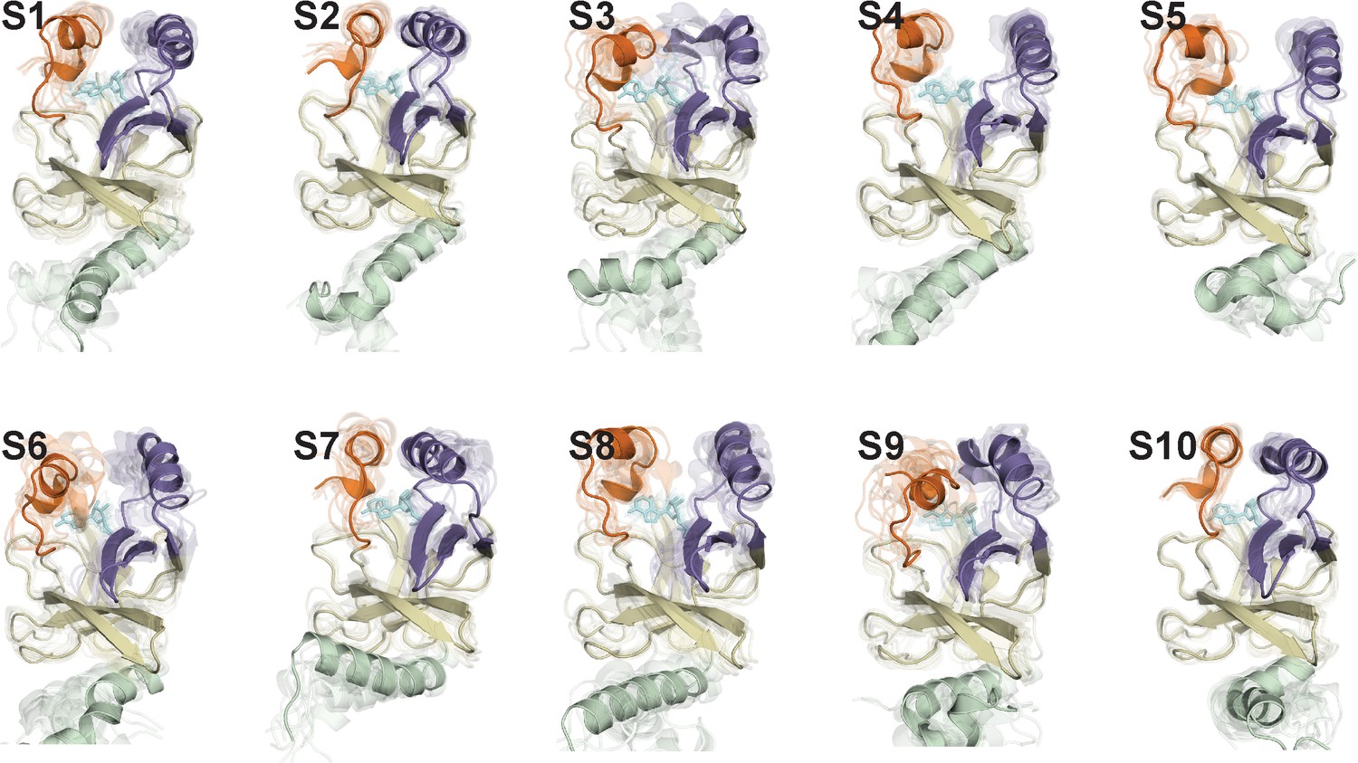
Representative conformations of macrostates in the conformational landscape of SAM-bound SETD8.
10 frames closest to the center of the microstate with the largest observation probability are presented.
Figure 6

Experimental design to probe the conformational landscape of SETD8.
(a) Comparison of binding environments of Trp390 (blue) between apo and SAM-bound (orange) SETD8 in the context of their dynamic conformational landscapes. (b) Illustration of rapid-quenching stopped-flow experiments. These experiments were conducted to trace fluorescence changes of Trp390 upon SAM binding. (c) Comparison of the conformations of post-SET kink and SET-I helix between apo- and SAM-bound SETD8 in the context of their dynamic conformational landscapes. Analysis of key structural motifs indicated K382P (blue in the upper panel), I293G and E292G (red in the lower panel) as potential gain-of-function variants.
Figure 7 with 3 supplements
Biochemical characterization of gain-of-function mutations revealed by conformational landscapes of SETD8.
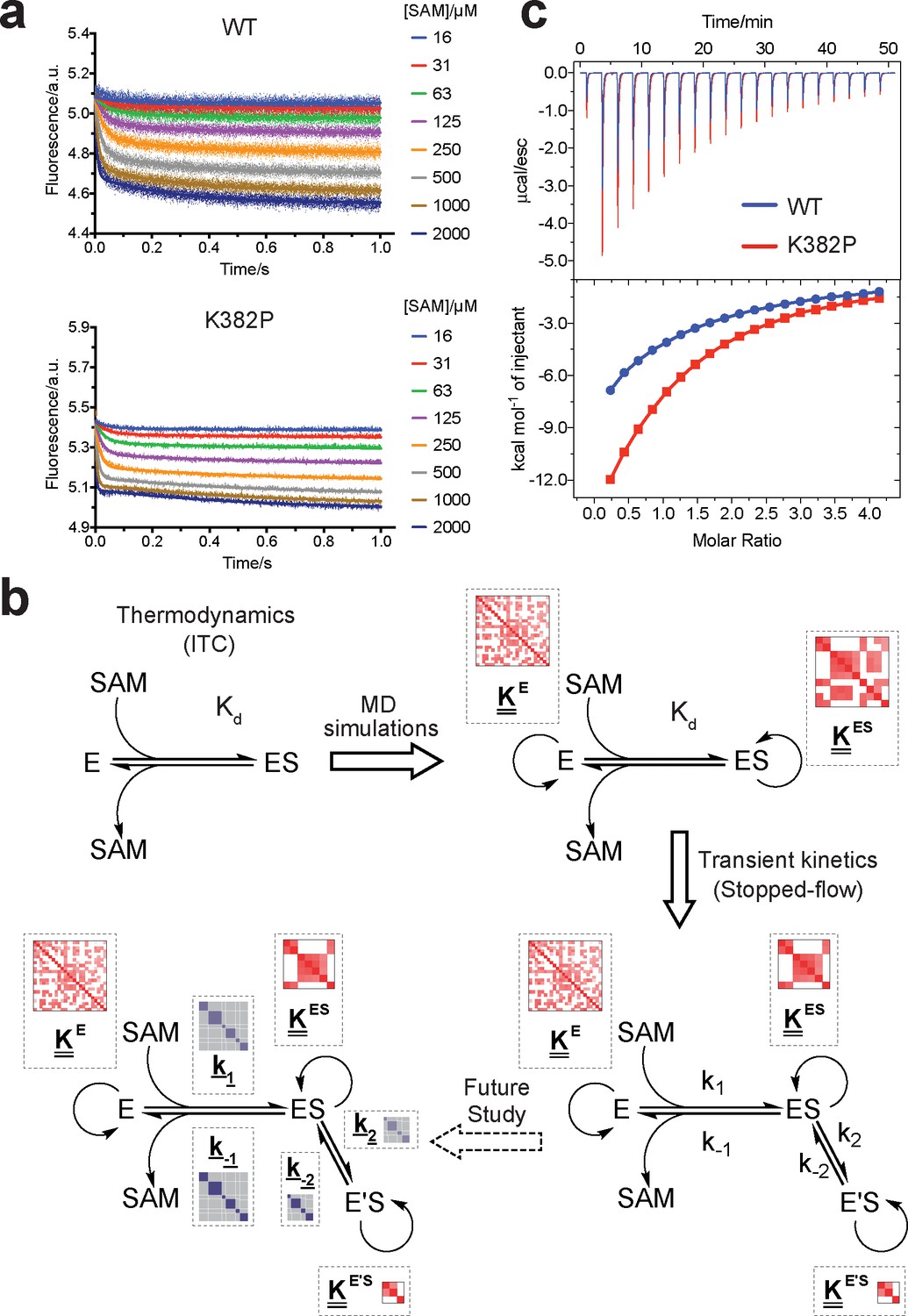
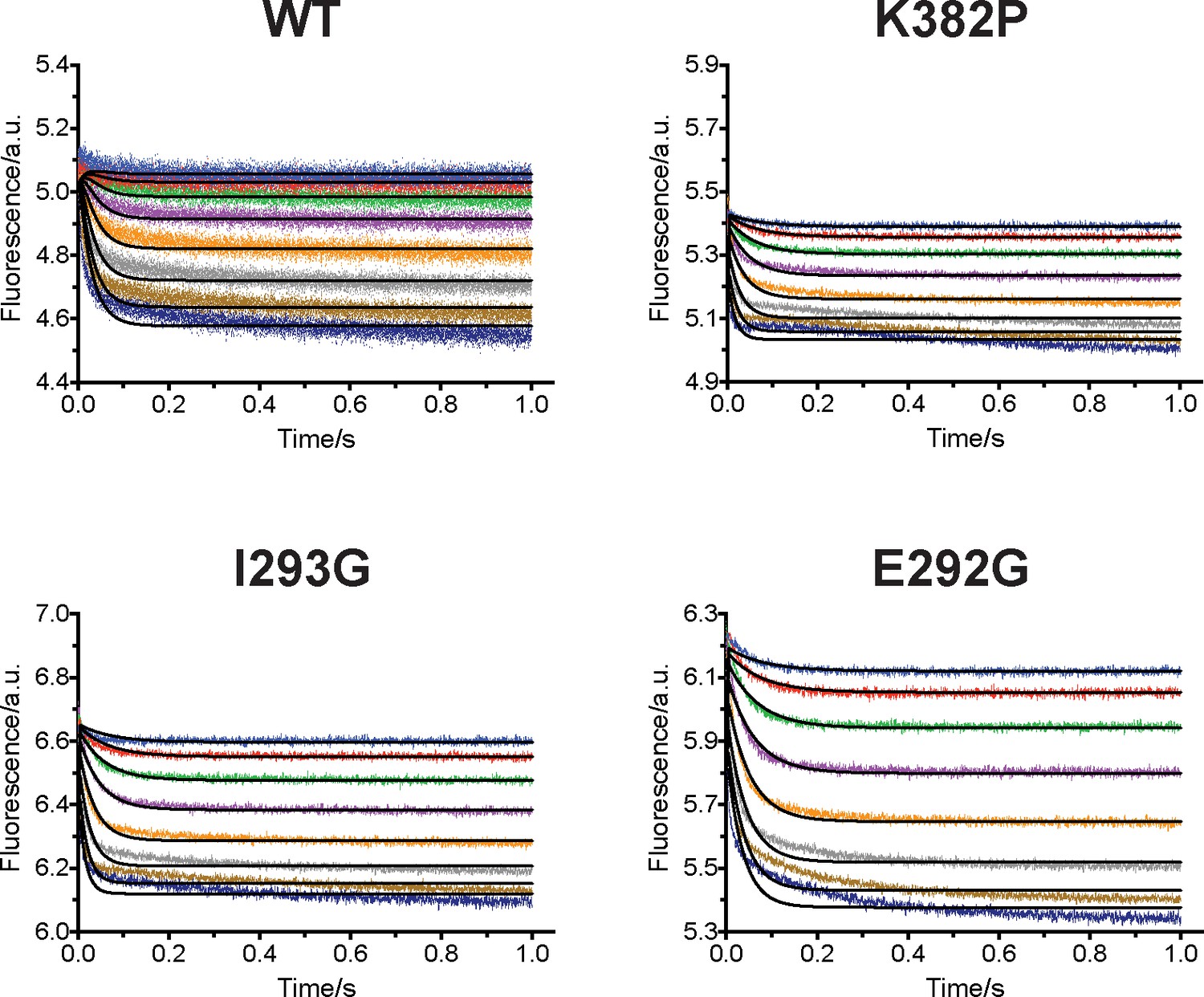
(a) Fluorescence changes of wild-type and K382P SETD8 traced with a rapid-quenching stopped-flow instrument within 1 s upon SAM binding. (b) Stepwise SAM-binding of SETD8 in the integrative context of biochemical, biophysical, structural, and simulation data. ITC determines the thermodynamic constant of SAM binding by SETD8. MD simulations and MSM uncover metastable conformations and interconversion rates of apo- and SAM-bound SETD8 (Kapo and KSAM). Stopped-flow experiments revealed that SETD8 binds SAM via biphasic kinetics. Rate constants uncovered by stopped-flow experiments (k1, k-1, k2, k-2) represent macroscopic rates of SAM binding by SETD8 with multiple metastable conformations. The microscopic behavior of individual metastable states and corresponding rates (k1, k-1, k2, k-2) have not been resolved. Transition probability matrices (red) and microscopic rate constant matrices (blue) are shown as colored grids. A rigorous mathematical derivation of this scheme is shown in Figure 7—figure supplement 3. (c) ITC enthalpogram for the titration of SAM into wild-type and K382P SETD8.
Figure 7—figure supplement 1
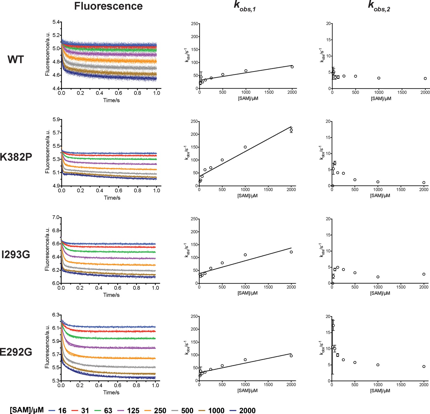
Rapid-mixing stopped-flow experiments of SAM-binding and double-exponential conventional fitting analysis.
Fluorescence decrease of SETD8 wild-type and designed mutants in SAM binding were determined by rapid-mixing stopped-flow experiments and analyzed by two-step global fitting (left column). The data were also conventionally fitted into a double-exponential equation, and two kobs are plotted against SAM concentration.
Figure 7—figure supplement 2
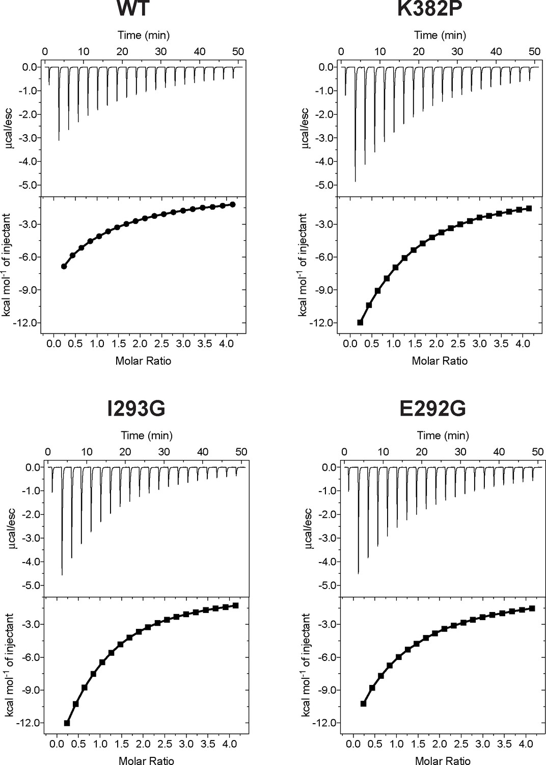
Isothermal Titration Calorimetry (ITC) of wild-type SETD8 and its mutants in complex with SAM.
Figures shown here are representatives of multiple replicates data.
Figure 7—figure supplement 3
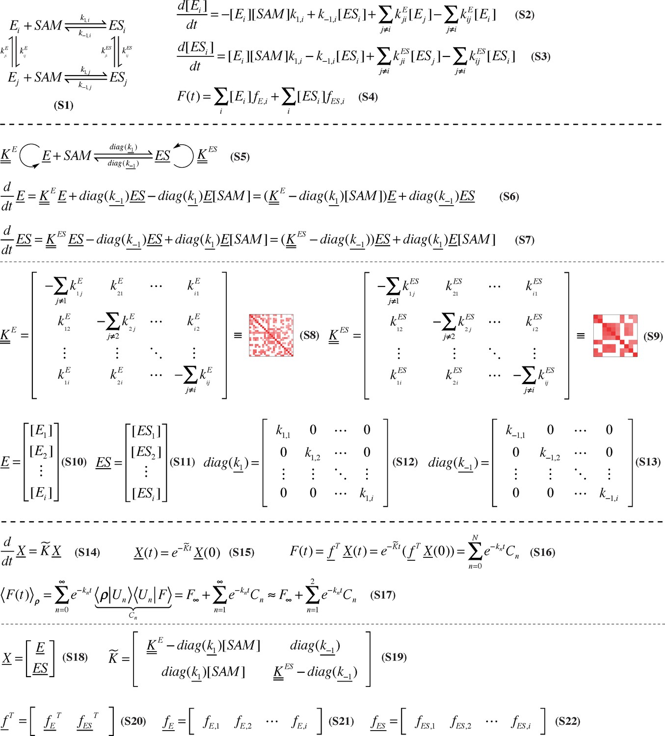
Rigorous derivation of stepwise, microscopic resolution of SETD8 SAM-binding kinetics.
A generalized kinetic mechanism for SAM binding that includes interconversion of apo- (E) and SAM-bound (ES) SETD8 among metastable conformational states is shown in Equation. S1. Equation. S2-S3 depict the corresponding kinetic model for time-evolution of apo- and SAM-bound populations in different conformational states, where the subscript i indexes conformational state. The time-dependent fluorescence signal can then be computed as a linear combination of the fluorescence of each species (Equation.S4). This kinetic model can be written in vectorial notation by writing the vector of populations of metastable conformational states as E (Equation. S10) and ES (Equation. S11), respectively (Equation. S5–S7), where rate constants are now denoted by matrices (Equation. S8–S9, S12–S13). Even more generally, populations for all chemical states can be gathered into a single vector X (Equation. S18) and the time-evolution and observed fluorescence for the entire system takes especially simple form (Equation. S14–S16). The observed fluorescence signal following rapid mixing can be decomposed into contributions from eigenfunctions |Un > and associated phenomenological rate constants kn (Equation. S17) arising from the dominant eigenvalues and associated eigenvectors of K (Equation. S19), and can be truncated to an equilibrium contribution (F∞) and the two dominant decay timescales if these processes dominate the eigenvalue spectrum of K.
Figure 8
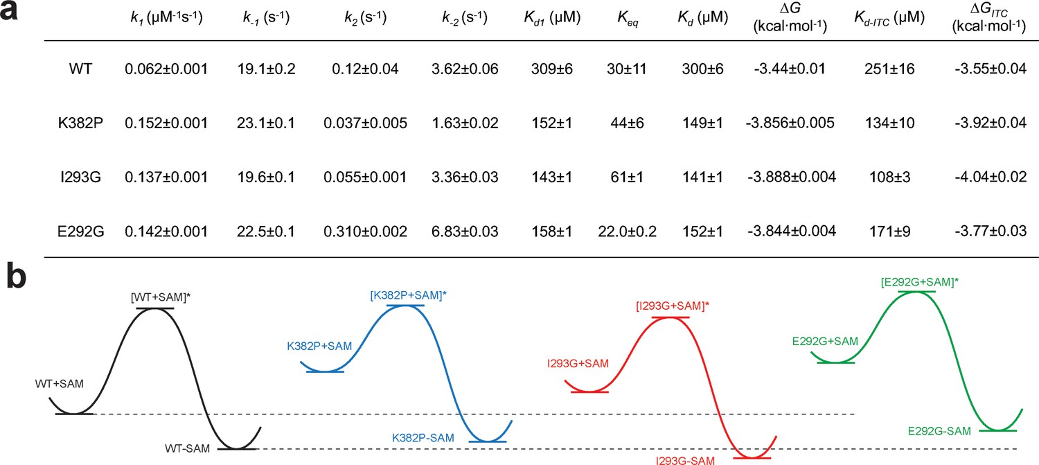
Kinetic and thermodynamic constants of wild-type SETD8 and its rationally designed mutants.
For k1, k-1, k2, k-2 in Figure 7, data are best fitting values ± standard error (s.e.) from KinTek. For Kd-ITC, data are mean ±s.e. of at least three replicates. Kd1, Keq, and Kd are calculated based on equations in Methods. Uncertainties of Kd1, Keq, Kd, and ΔG are s.e. calculated by the propagation of uncertainties from individual rate constants and dissociation constants, respectively. h, Relative energy landscapes of apo- and SAM-bound SETD8 and its gain-of-function mutants. The relative energy of apo- and SAM-bound (wildtype and mutated) SETD8 as well as their transition states were determined on the basis of their k1, k-1, and Kd values. The relative position of each energy landscape was then set on the basis of the rough counts of mutation-associated loss or gain of favorable interactions in contrast to apo- or SAM-bound wild-type SETD8. All SETD8 variants except SAM-bound I293G disrupt the favorable interactions to various degrees.
Figure 9
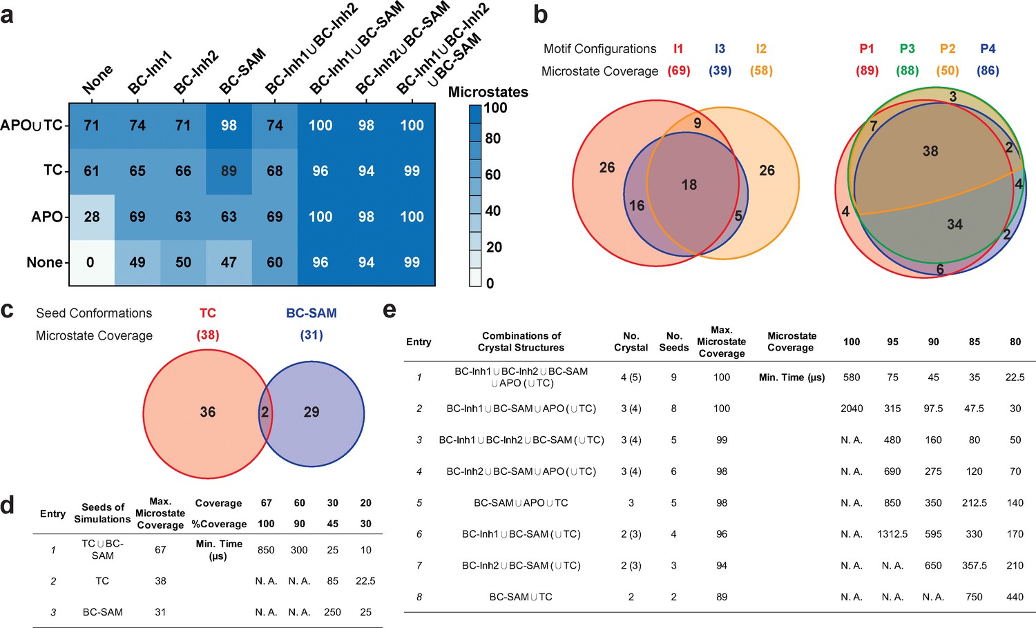
Evaluation of key simulation parameters of molecular simulations.
(a−b) Assessments of simulations of apo-SETD8: (a) Heat map for the coverage of the 100 microstates with all combinations of the crystal structures (BC-Inh1, BC-Inh2, BC-SAM, APO, and TC) as seed conformations; (b) Venn diagrams of the coverage of the 100 microstates with all conformational combinations of SET-I and post-SET motifs (I1-3 and P1-4) as seed structures for MD simulations. (c−d) Robustness of simulations of SAM-bound SETD8: (c) Venn diagram of the coverage of the 67 microstates with TC, BC-SAM or both as seed structures for MD simulation; (d) Minimal time required by MD simulations to reach certain coverage of the 67 microstates of SAM-bound SETD8 with representative combinations of seed structures. (e) Minimal time required by MD simulations to reach certain coverage of the 100 microstates of apo-SETD8 with representative combinations of seed structures.
Figure 10 with 1 supplement
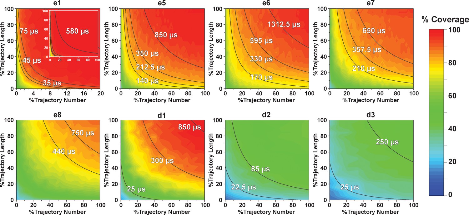
Contour map of microstate coverage at various combinations of trajectory lengths and numbers as percentage of the maximal trajectory length and number of MD simulations.
The seed structures of each panel are listed as the simulation entries e1, e5−8 for apo-SETD8, and d1−3 for SAM-bound SETD8 in Figure 9d and e. Each curve corresponds to the aggregation of specific simulation time.
Figure 10—figure supplement 1
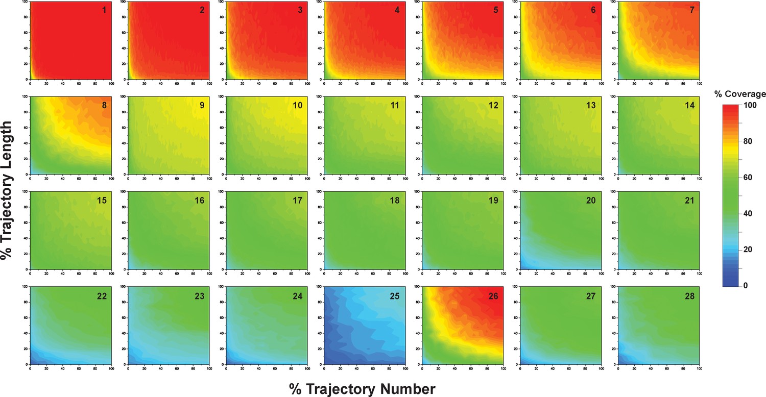
Contour maps presenting microstate coverage at various trajectory lengths and numbers versus the maximal possible trajectory length or number at different combinations of starting conformations.
The combinations are numbered as listed in Supplementary file 1o, 1p. Similar microstate coverage at same aggregate simulation time but different trajectory numbers/lengths indicate these two factors alone do not have obvious influence on the coverage of microstates.
Figure 11
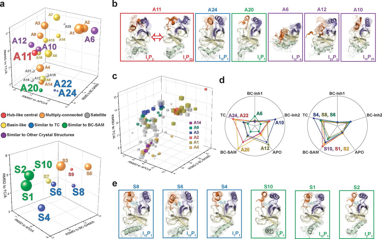
Functional annotation of the dynamic conformational landscapes of SETD8.
(a) 3D scatterplots of the 24 macrostates of apo-SETD8 landscape and 10 macrostates of SAM-bound SETD8 landscape in the coordinates of RMSDs relative to APO, BC-SAM, and TC. Volume of each sphere is proportional to the relative population of the corresponding macrostate in the context of the 24 macrostates for apo-SETD8 or the 10 macrostates for SAM-bound SETD8. The RMSD of each macrostate is the average of its microstates weighted with their intra-macrostate populations. The RMSD of each microstate is the average of the top 10 frames most closely related to the clustering center of the microstate. The feature of each macrostate is annotated in color. (b) Cartoons of representative conformations of key macrostates in the apo-SETD8 landscape. Structural annotations are shown in bottom right of each conformation. (c) 3D scattering plot of 100 microstates of the apo landscape in the coordinates of RMSDs to APO, BC-SAM, and TC. Volume of each cube is proportional to the relative population of the corresponding microstate in the context of the 100 microstates. Microstates clustered in intermediate-like macrostates are highlighted in colors. Structural diversity of microstates within individual macrostates indicates that each intermediate-like state contains multiple structurally distinct but readily interconvertible microstates. (d) Radar chart of representative macrostates of apo (left) and SAM-bound (right) landscapes in reference to the five crystal structures. Distances between dots and cycle centers are proportional to the reciprocal values of RMSDs of macrostates relative to the crystal structures. (e) Cartoons of representative conformations of key macrostates in the SAM-bound SETD8 landscape. Structural annotations are shown in bottom right of each conformation.
Figure 12 with 2 supplements
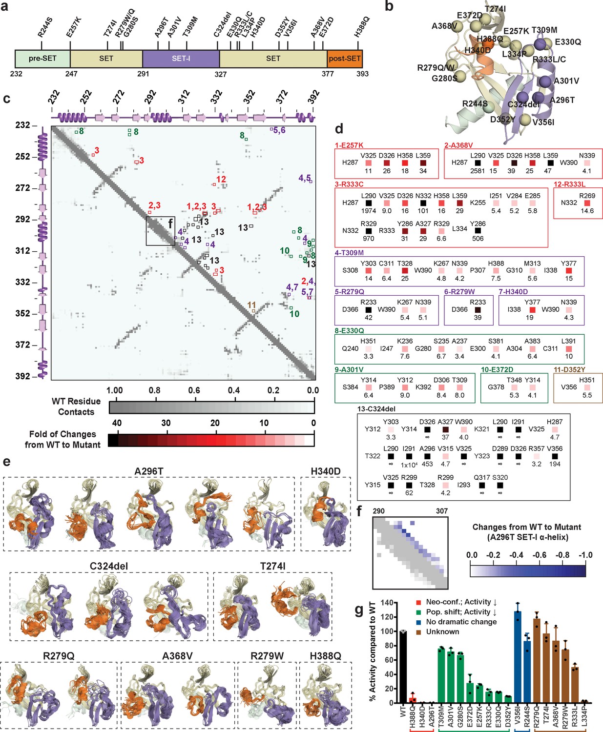
Computational and experimental characterization of cancer-associated SETD8 mutants.
(a) Cancer-associated mutations in the catalytic domain of SETD8 examined in this work. (b) Cartoon representations of TC with cancer-associated SETD8 mutations highlighted. (c) Differential residue-contact maps of cancer-associated SETD8 mutants in reference to wild-type apo-SETD8 (gray). Residue-residue contact map of wild-type apo-SETD8 is presented as a 162 × 162 matrix. The vertical and horizontal axes show the residue numbers of SETD8’s catalytic domain. The contact of a pair of residues is scored as ‘1’ if their distance is shorter than 4.0 Å; ‘0’ if the distance is equal or above 4.0 Å. For the 60 1ZKK(chain A)-seeded MD trajectory frames of wild-type apo-SETD8, the average contact fraction of each residue pair is presented in a square shape and depicted with a gray gradient at the corresponding vertical and horizontal coordinates. The contact fraction of cancer-associated SETD8 mutants were obtained in a similar manner. The vertical and horizontal coordinates of representative positive changes of the contact scores from wild-type to mutated SETD8 (newly acquired interactions) are highlighted in red-gradient squares with details expanded in the next panel. (d) Representative contacts in the differential residue-contact maps of cancer-associated SETD8 mutants. The contacts of SETD8 mutants with >3 fold gain of contact fraction relative to wild-type SETD8 are listed. Increased magnitude of the contact fraction is depicted in red gradient as described in the previous panel. Only positive changes (newly acquired interactions) are presented with the two residues involved labeled in left and top; the fold of the increase of their contact score labeled in bottom. (e) Cartoon representations of neo-conformations revealed by simulations of SETD8 mutants. Large conformational changes are observed in the SET-I (purple) and post-SET (orange) motifs. (f) Differential residue-contact maps of the structurally relaxed α-helix at the SET-I motif of SETD8 A296T mutant. Decrease of contact fraction relative to wild-type SETD8 is depicted in blue gradient. (g) Enzymatic activities of wild-type and mutated SETD8 determined by an in vitro radiometric assay with H4K20 peptide substrate. Here SETD8 mutants are categorized as the following: red, uncovered neo-conformations (Neo-conf.) with >90% loss of methyltransferase activity; green, populated inactive conformations (Pop. shift) with partially abolished methyltransferase activity; blue, no large change of differential contact maps with comparable methyltransferase activity with wild-type SETD8; brown, unknown relationship between differential contact maps and methyltransferase activities. Data are mean ±standard deviation (s.d.) of 3 replicates.
Figure 12—figure supplement 1
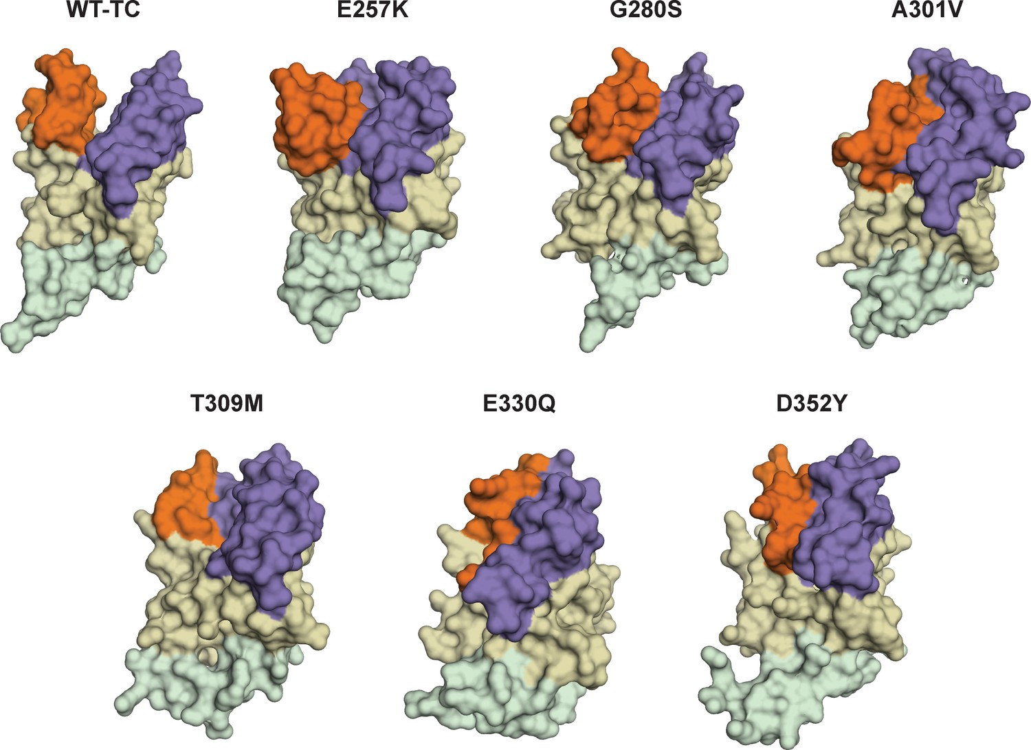
Cartoon representations of cancer-associated SETD8 variants with more populated inactive conformations.
Representative frames from MD simulations of some SETD8 cancer-associated mutants (E257K, G280K, A301V, T309M, E330Q, D352Y) shows compression of active site pockets. Conformation of TC) of wild-type SETD8 is also shown here (WT-TC). Orientation of view is the same as used in Figure 1.
Figure 12—figure supplement 2
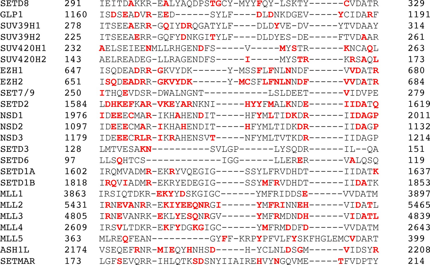
Cancer-associated mutations in the SET-I region of PKMTs reported in cBioPortal.
Protein sequences of PKMTs are overlaid, and the regions aligned with the SET-I motif of SETD8 are shown. Amino acid residues with cancer-associated mutations identified in cBioPortal are highlighted in red.
Appendix 1—figure 1
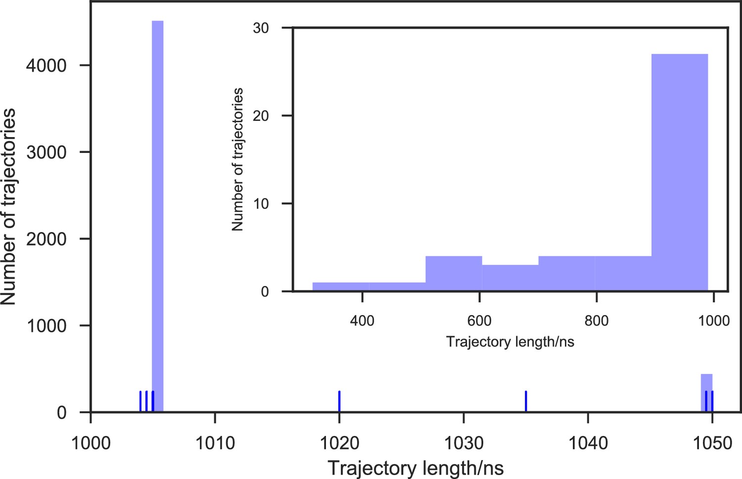
Distribution of trajectory lengths of apo-SETD8 simulation.
5,020 Trajectories were collected in total. 99.1% of these trajectories (4,976 trajectories) reached at least 1 μs of simulation time, resulting in 5.058 ms of aggregate simulation time.
Appendix 1—figure 2
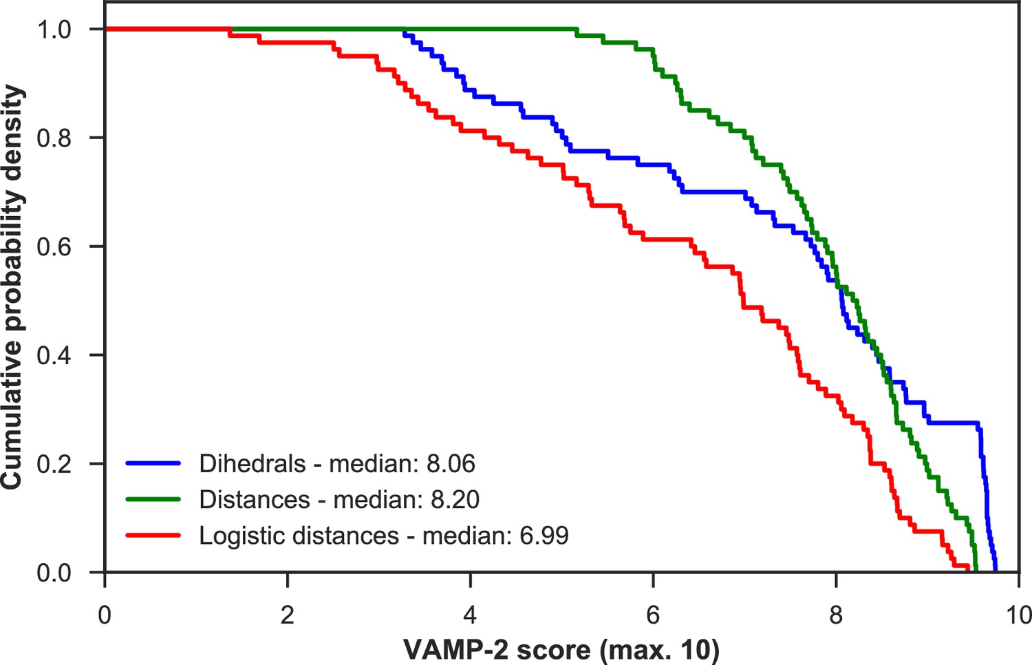
VAMP-2 scoring results for optimal hyperparameter choice for featurization and tICA.
For each featurization, the empirical cumulative distribution functions of VAMP-2 scores (from highest to lowest) for all other hyperparameter choices combined are shown. On the basis of the medians of all scores, the distance features perform the best.
Appendix 1—figure 3
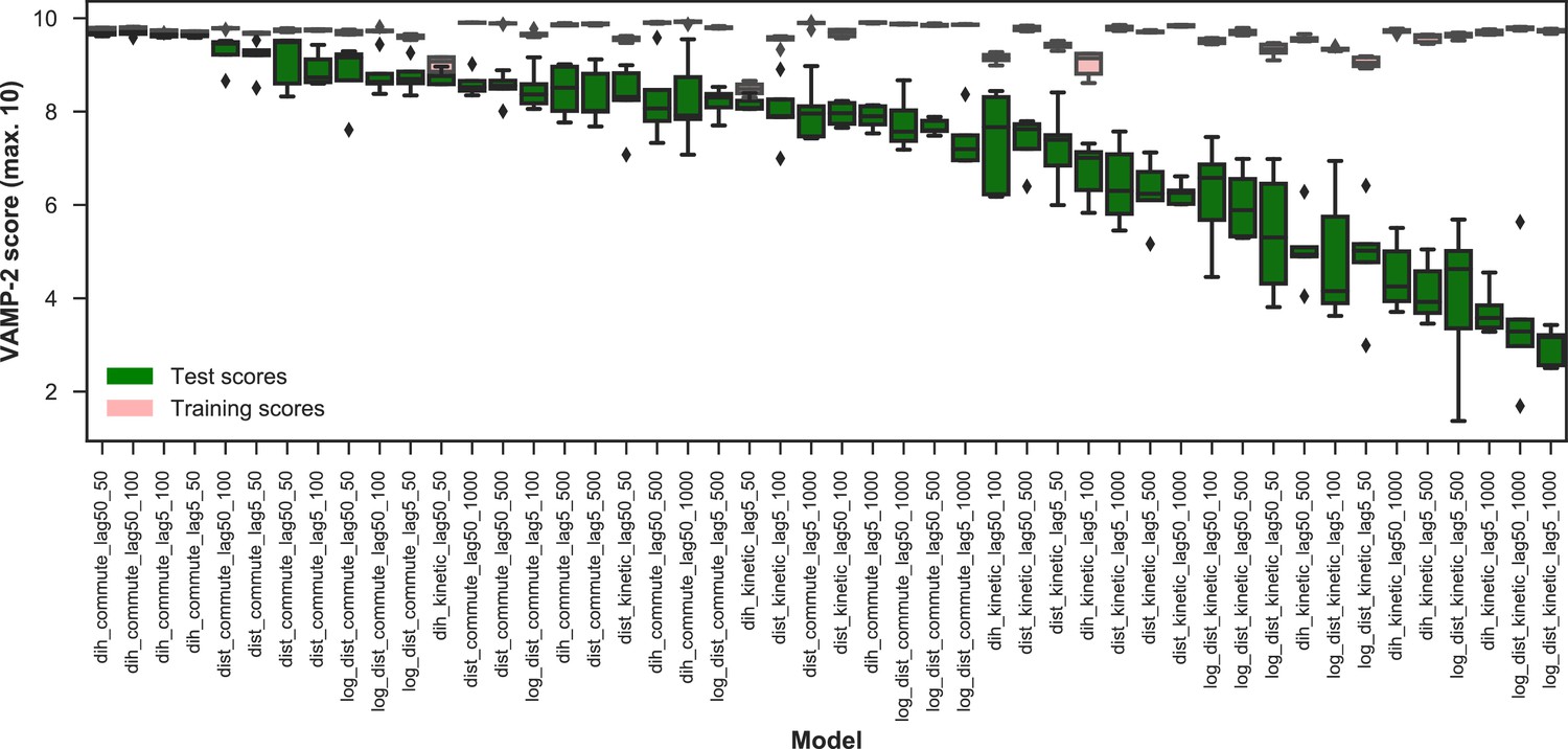
VAMP-2 scoring results for optimal hyperparameter choice for featurization and tICA.
The distributions of VAMP-2 scores of five shuffle-splits of the data for each individual set of hyperparameters (model) are shown as box-and-whisker plots. Bands of boxes show the first, second, and third quartiles, while whisker ends represent the lowest and highest scores still within 1.5 of the interquartile range from the first and third quartiles respectively. Scores lying outside of that range are shown as diamonds. The models are denoted as {featurization}_{tICA mapping}_{tICA lag time (in ns)}_{number of microstates}, where the featurization is one of ‘dih’ for dihedrals, ‘dist’ for distances, or ‘log_dist’ for logistic distances. Test scores are shown in green and training scores in red. On the basis of the highest scoring individual model, the dihedral features, which were used for the four top scoring models, perform the best.
Appendix 1—figure 4

VAMP-2 scoring results for optimal hyperparameter choice for tICA with dihedral features.
The distributions of test scores of all microstate number choices for all combinations of tICA mapping and lag times are shown as box-and-whisker plots. Bands of boxes show the first, second, and third quartiles, while whisker ends represent the lowest and highest scores still within 1.5 of the interquartile range from the first and third quartiles respectively. The models are described as {featurization}_{tICA lag time (in ns)}. Commute mapping performs significantly better than kinetic mapping and there is no significant difference in performance between the two lag times when commute mapping is used.
Appendix 1—figure 5
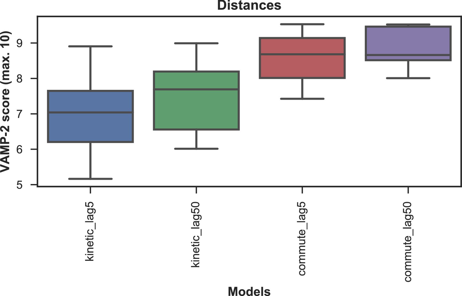
VAMP-2 scoring results for optimal hyperparameter choice for tICA with distance features.
The distributions of test scores of all microstate number choices for all combinations of tICA mapping and lag times are shown as box-and-whisker plots. Bands of boxes show the first, second, and third quartiles, while whisker ends represent the lowest and highest scores still within 1.5 of the interquartile range from the first and third quartiles respectively. The models are described as follows: {tICA mapping}_{tICA lag time (in ns)}. Commute mapping performs significantly better than kinetic mapping and there is no significant difference in performance between the two lag times when commute mapping is used.
Appendix 1—figure 6
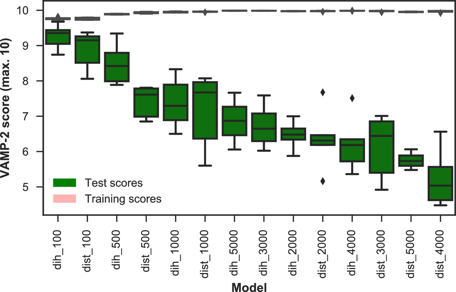
VAMP-2 scoring results for final featurization and microstate number choice.
The distributions of scores of five shuffle-splits of the data for all combinations of dihedrals or distances featurization and the numbers of microstates are shown as box-and-whisker plots. Bands of boxes show the first, second, and third quartiles, while whisker ends represent the lowest and highest scores still within 1.5 of the interquartile range from the first and third quartiles respectively. Scores lying outside of that range are shown as diamonds. The models are described as follows: {featurization}_{number of microstates}. Featurizations are denoted by ‘dih’ for dihedrals or ‘dist’ for distances. Test scores are shown in green and training scores in red (due to the narrowness of the boxes for the training scores the color is not visible). The highest scoring model has dihedral features and 100 microstates.
Appendix 1—figure 7
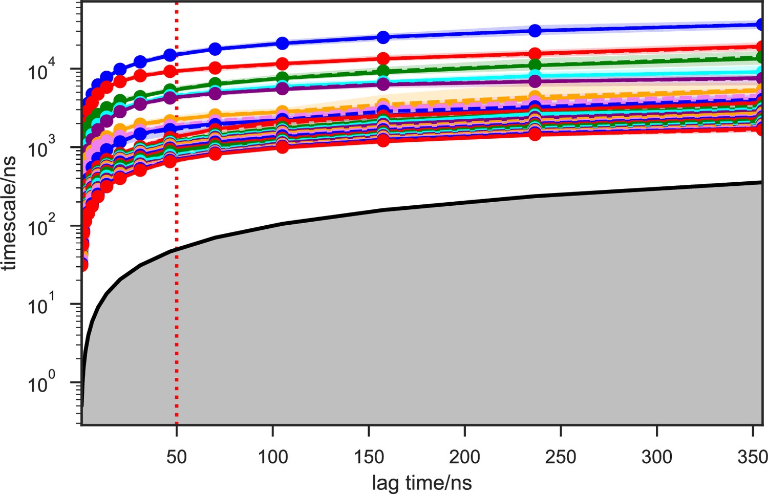
Implied timescales of the apo-SETD8 Bayesian Markov state models (BMSMs).
The top 23 implied timescales (corresponding to 24 macrostates) of the BMSMs calculated at a range of lag times are shown: the maximum likelihood estimates (MLEs) as solid lines, the means as dashed lines, and the 95% confidence intervals of the means as shaded regions. The gray area signifies the region where timescales become equal to or smaller than the lag time and can no longer be resolved. The lag time of 50 ns (marked by the dashed red vertical line) is chosen for our models, as the timescales have approximately leveled off at that point.
Appendix 1—figure 8
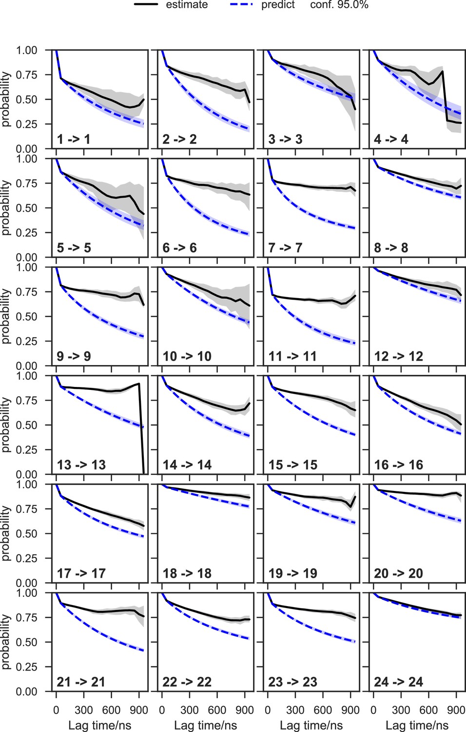
Chapman-Kolmogorov test of the apo-SETD8 Bayesian Markov state model (BMSM) using the metastable memberships from the Hidden Markov state model (HMM).
The objective of the Chapman-Kolmogorov test is to assess the kinetic self-consistency of the MSM, i.e., whether the predictions of longer time behavior made from the BMSM being tested match the estimates made from BMSMs generated at longer lag times. For each HMM macrostate, probability density is assigned to the BMSM microstates according to their metastable memberships to the given macrostate and evolution of the probability in time in the tested BMSM is plotted in blue. At those same longer lag times new BMSMs are estimated and their probability densities of being in the given macrostate are plotted in black. The shaded regions correspond to the 95% confidence intervals of the mean of the predictions and estimates. In this case, our model does not faithfully reproduce the empirically-observed slow escape times for many of the macrostates, meaning that insufficient data is available for a quantitative reproduction of the inter-state kinetics; despite this, the equilibrium populations of the macrostates and qualitative resolution of low and high interstate fluxes can still be estimated with good fidelity.
Appendix 1—figure 9

Implied timescales of the apo-SETD8 Bayesian Hidden Markov state models (BHMSMs).
The top 23 implied timescales (corresponding to 24 macrostates) of the BHMSMs calculated at a range of lag times are shown: the maximum likelihood estimates (MLEs) as solid lines, the means as dashed lines, and the 95% confidence intervals of the means as shaded regions. The gray area signifies the region where timescales become equal to or smaller than the lag time and can no longer be resolved. The lag time of 50 ns (marked by the dashed red vertical line) is chosen for our models, as the timescales have approximately leveled off at that point.
Appendix 1—figure 10
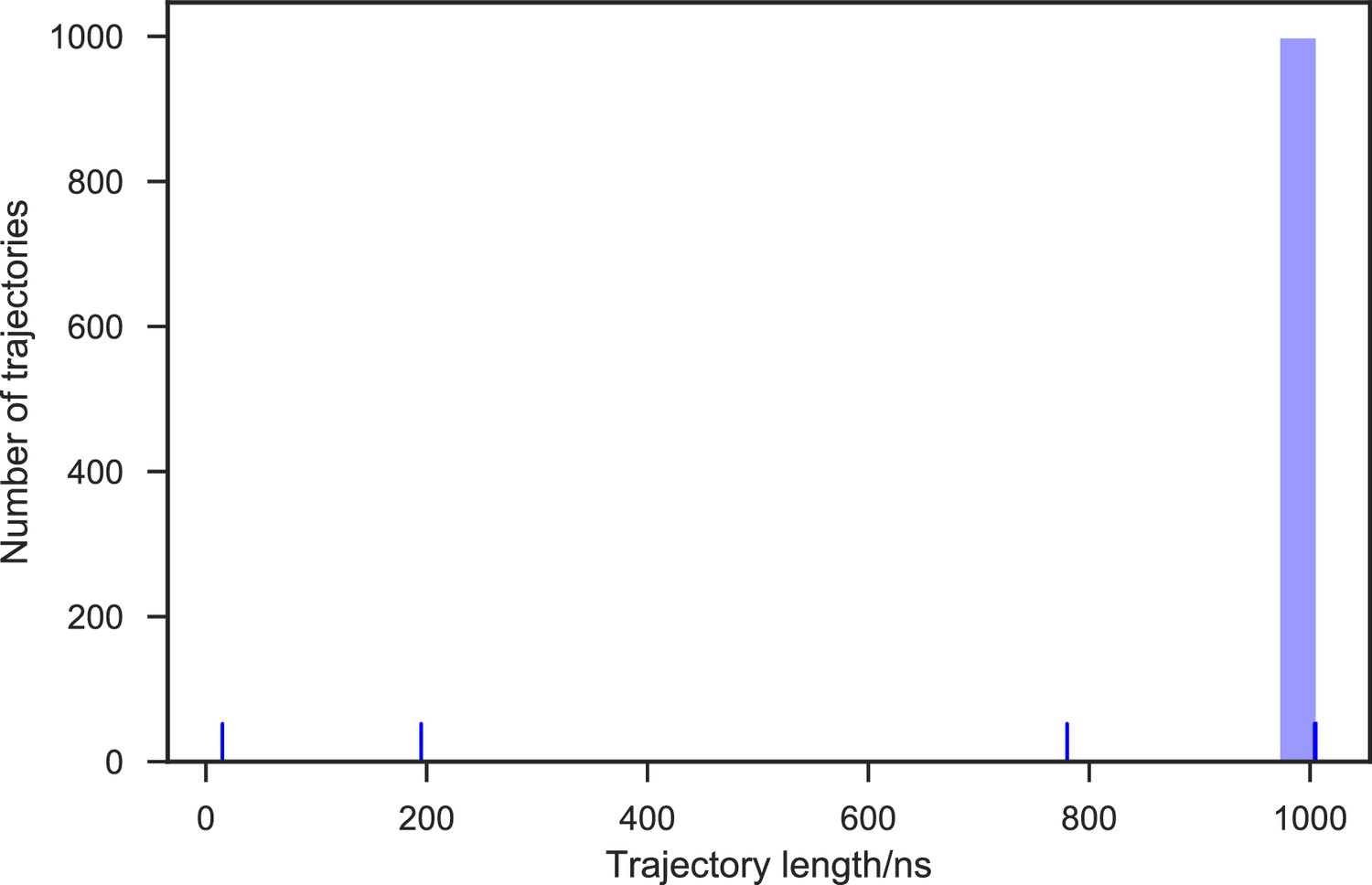
Distribution of the SAM-bound SETD8 simulation trajectory lengths.
1,000 trajectories were collected in total. 99.7% of the 1,000 trajectories (997 trajectories) reached at least 1 μs of simulation time, resulting in 1.003 ms of aggregate simulation time.
Appendix 1—figure 11
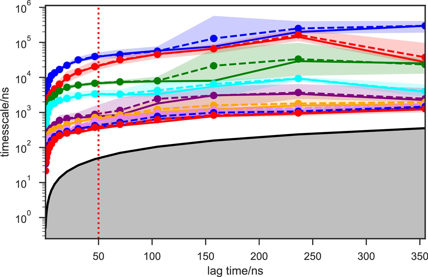
Implied timescales of the SAM-bound SETD8 Bayesian Markov state models (BMSMs).
The top 9 implied timescales (corresponding to 10 macrostates) of the BMSMs calculated at a range of lag times are shown: the maximum likelihood estimates (MLEs) as solid lines, the means as dashed lines, and the 95% confidence intervals of the means as shaded regions. The gray area signifies the region where timescales become equal to or smaller than the lag time and can no longer be resolved. The lag time of 50 ns (marked by the dashed red vertical line) is chosen for our models, as the timescales have approximately leveled off at that point.
Appendix 1—figure 12
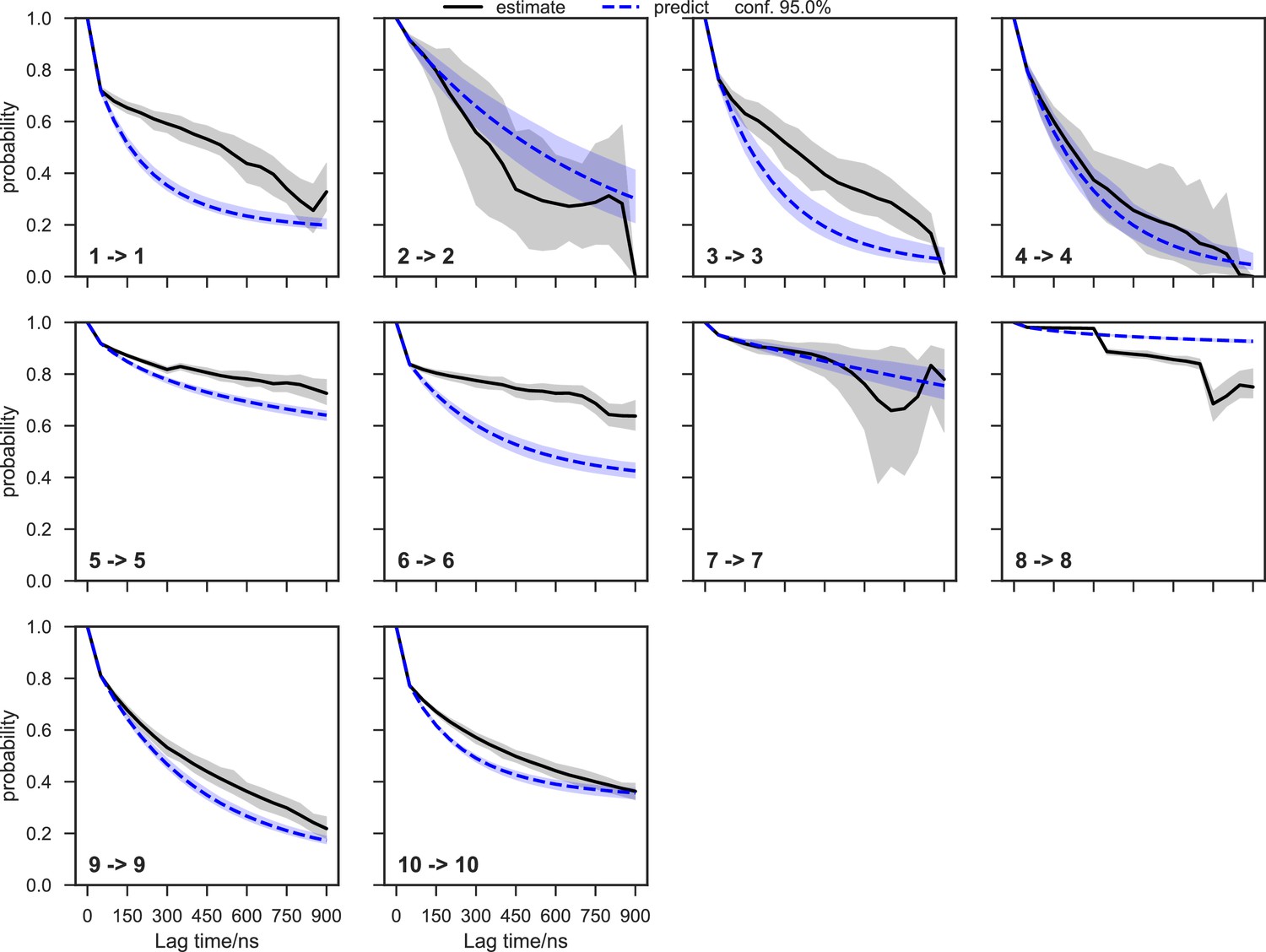
Chapman-Kolmogorov test of the SAM-bound SETD8 Bayesian Markov state model (BMSM) using the metastable memberships from the Hidden Markov state model (HMM).
The objective of the Chapman-Kolmogorov test is to assess the kinetic self-consistency of the MSM, i.e., whether the predictions of longer time behavior made from the BMSM being tested match the estimates made from BMSMs generated at longer lag times. For each HMM macrostate, probability density is assigned to the BMSM microstates according to their metastable memberships to the given macrostate and evolution of the probability in time in the tested BMSM is plotted in blue. At those same longer lag times new BMSMs are estimated and their probability densities of being in the given macrostate are plotted in black. The shaded regions correspond to the 95% confidence intervals of the mean of the predictions and estimates. In this case, our model does not faithfully reproduce the empirically-observed slow escape times for many of the macrostates, meaning that insufficient data is available for a quantitative reproduction of the inter-state kinetics; despite this, the equilibrium populations of the macrostates and qualitative resolution of low and high interstate fluxes can still be estimated with good fidelity.
Appendix 1—figure 13
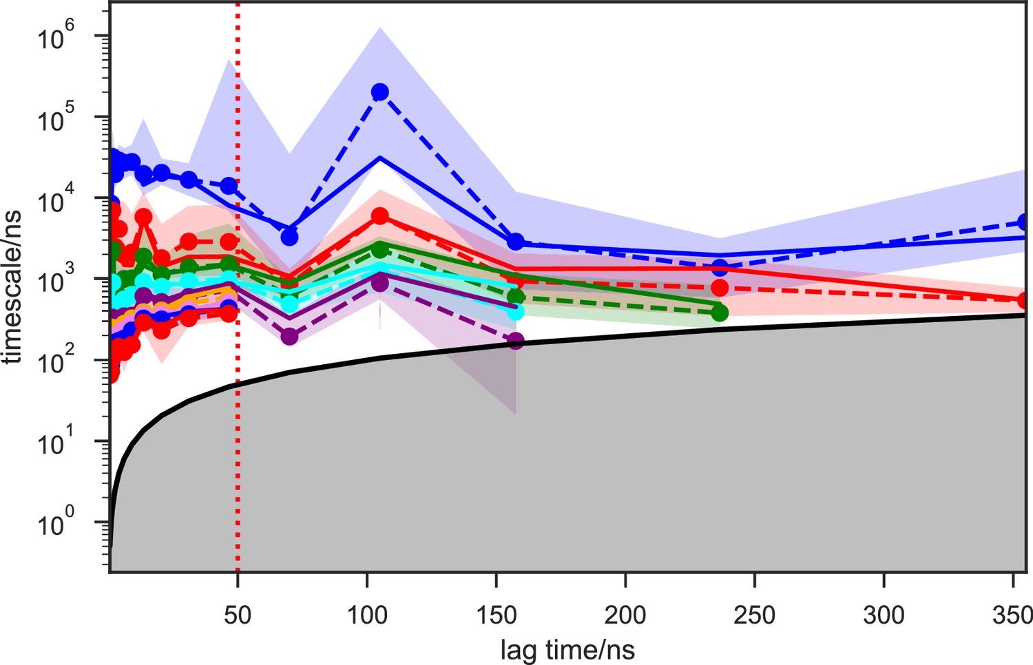
Implied timescales of the SAM-bound SETD8 Bayesian Hidden Markov state models (BHMSMs).
The top 9 implied timescales (corresponding to 10 macrostates) of the BHMSMs calculated at a range of lag times are shown: the maximum likelihood estimates (MLEs) as solid lines, the means as dashed lines, and the 95% confidence intervals of the means as the shaded regions. The gray area signifies the region where timescales become equal to or smaller than the lag time and can no longer be resolved. The lag time of 50 ns (marked by the dashed red vertical line) is chosen for our models, as the timescales have approximately leveled off at that point.
Appendix 1—figure 14
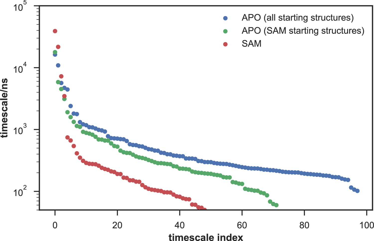
Comparison of the kinetic complexity of apo- and SAM-bound SETD8.
All timescales larger than the Markovian lag time (50 ns) are shown for Markov state models built using: all apo trajectories (5,019 trajectories), all SAM-bound trajectories (1,000 trajectories), and the subset of apo trajectories starting from the same conformations as SAM-bound trajectories (1,200 trajectories). There is a large decrease in the number of slow processes seen in the SAM-bound model compared to the other two (respectively for the apo, SAM-bound, and subset of apo MSMs there are 14, 4, and 9 processes slower than 1 μs).
Appendix 1—figure 15
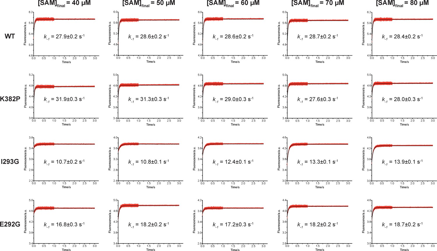
Rapid-mixing stopped-flow dilution of SAM-bound SETD8.
Fluorescence increase of pre-incubated SETD8-SAM binary complex was determined by rapid-mixing stopped-flow dilution experiments with various final SAM concentrations and analyzed by one-exponential conventional fitting. Given the small fraction of second step in the SAM-binding process, the kobs mainly reflect k-1. Data are best fitting values ± s.e. from KinTek.
Appendix 1—figure 16
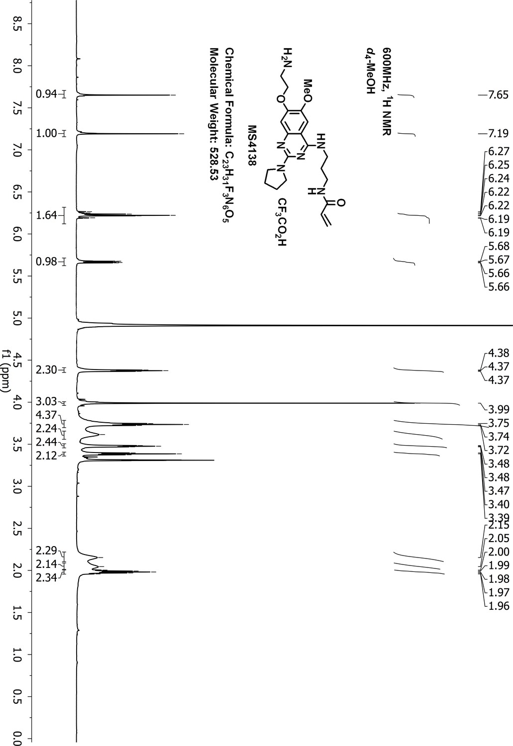
1H-NMR of MS4138 (Inh1).
https://doi.org/10.7554/eLife.45403.051
Appendix 1—figure 17
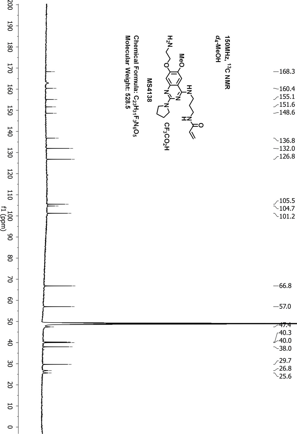
13C-NMR of MS4138 (Inh1).
https://doi.org/10.7554/eLife.45403.052
Appendix 1—figure 18
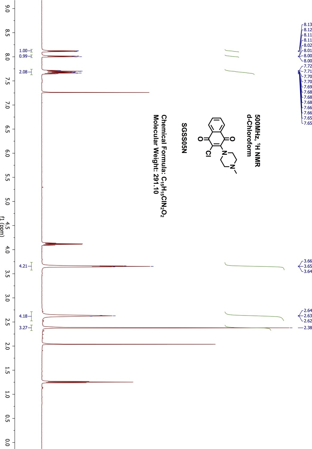
1H-NMR of SGSS05N.
https://doi.org/10.7554/eLife.45403.053
Appendix 1—figure 19
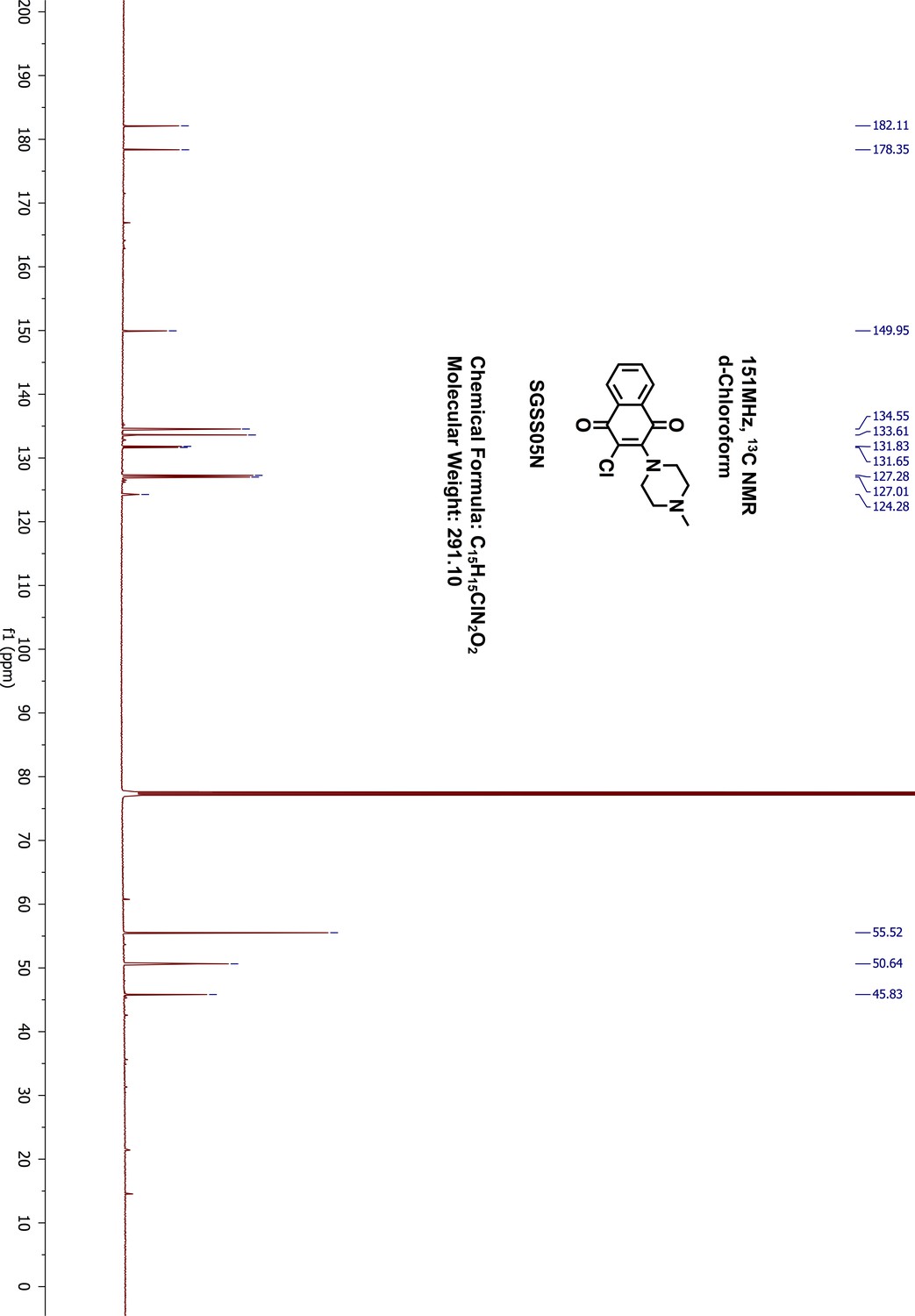
13C-NMR of SGSS05N.
https://doi.org/10.7554/eLife.45403.054
Appendix 1—figure 20
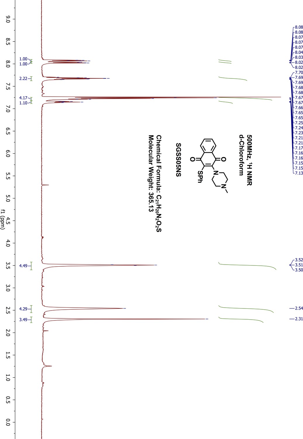
1H-NMR of SGSS05NS (Inh2).
https://doi.org/10.7554/eLife.45403.055
Appendix 1—figure 21
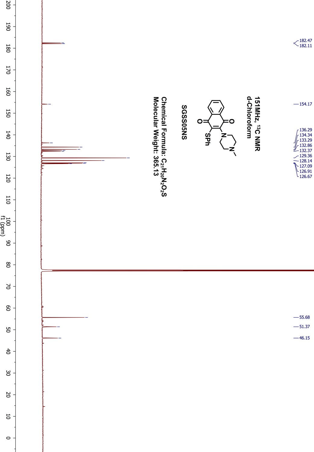
13C-NMR of SGSS05NS (Inh2).
https://doi.org/10.7554/eLife.45403.056
Appendix 1—figure 22
Global fitting analysis of stopped-flow binding experiment into a conformational selection model.
In contrast to the model we proposed, global fitting analysis of fluorescence decreases from stopped-flow binding experiments into a conformational-selection model (E = E'+SAM = E'SAM) failed to generate good fitting results.
Appendix 1—figure 23
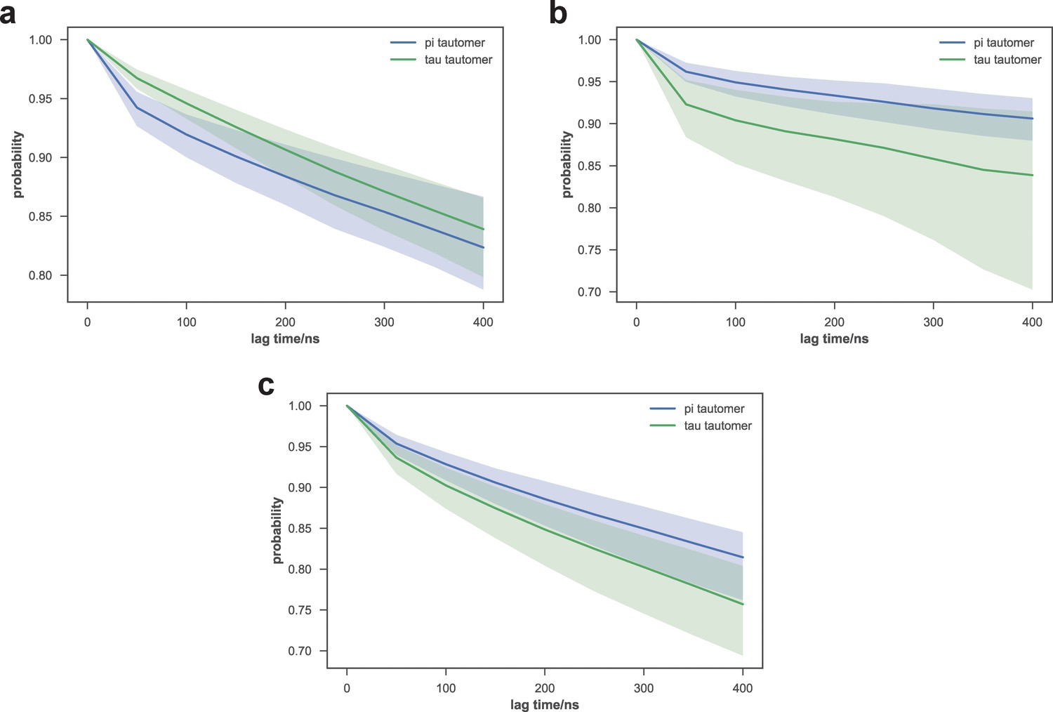
Comparison of macrostate escape kinetics for different His351 tautomers of apo-SETD8.
As subsets of initial models used for apo-SETD8 simulations used different His351 tautomers, we examined the kinetics of escape from several macrostates that were highly populated by both sets of trajectories. The probabilities of remaining in macrostates A9 (top), A1 (middle), and A4 (bottom) after a given lag time are shown. Means of 40 bootstraps are depicted as solid lines, with 95% confidence intervals shown as shaded regions.
Appendix 1—figure 24

Distribution of the 24 mutant apo-SETD8 simulation trajectory lengths.
960 trajectories were collected in total. 99.7% of them (957 trajectories) reached at least 1 μs in length, resulting in 0.966 ms of aggregate simulation time.
Appendix 1—figure 25
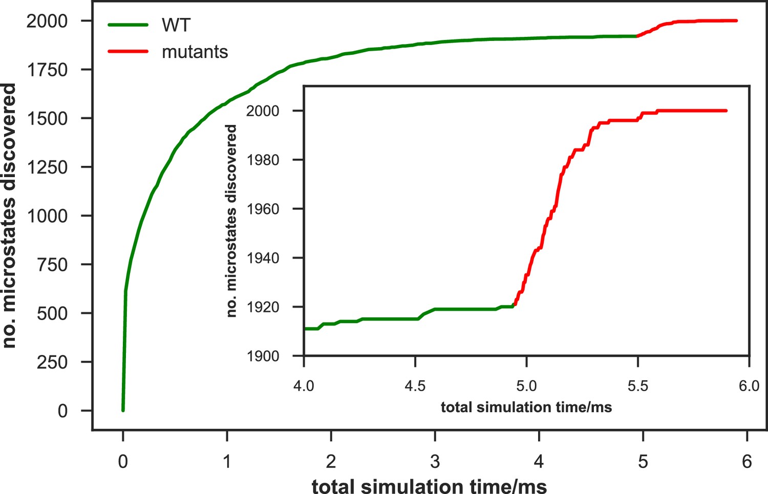
Rate of discovery of new microstates in wild-type (WT) and mutant apo-SETD8 datasets.
The number of microstates discovered as a function of cumulative aggregate simulation time (corresponding to a uniform initial fraction of all trajectories in the dataset) are shown for a 2,000 joint microstate clustering of the combined WT + mutants apo-SETD8 dataset. The WT data is shown in green, and the mutant data in red, appended to the WT curve for easy comparison. The inset plot shows the number of new microstates discovered for equal amounts of data (~1 ms aggregate simulation time) from the final portion of the WT trajectories and from mutant trajectories. The mutant dataset rapidly discovers 79 new microstates at a rate that far outstrips the discovery rate of new wild-type conformations.
Videos
Video 1
A 2 ms molecular dynamics trajectory simulated from the HMM of apo-SETD8.
https://doi.org/10.7554/eLife.45403.031
Video 2
A 2 ms molecular dynamics trajectory simulated from the HMM of SAM-bound SETD8.
https://doi.org/10.7554/eLife.45403.032Tables
Table 1
Data collection and refinement statistics of crystallography.
https://doi.org/10.7554/eLife.45403.010| BC-Inh1 | BC-Inh2 | BC-SAM | APO | |
|---|---|---|---|---|
| PDB Code | 6BOZ | 5W1Y | 4IJ8 | 5V2N |
| Data collection | ||||
| Wavelength (Å) | 0.98 | 0.98 | 0.98 | 0.98 |
| Space group | P212121 | P212121 | P6122 | P43212 |
| Cell dimensions | ||||
| a, b, c (Å) | 31.56, 68.06, 125.90 | 58.35, 39.79, 131.90 | 101.44, 101.44,140.80 | 60.6, 60.6, 80.7 |
| α, β, γ (°) | 90, 90, 90 | 90, 90, 90 | 90, 90, 120 | 90, 90, 90 |
| Resolution (Å) | 62.95–2.40 (2.49–2.40) | 43.70–1.70 (1.73–1.70) | 47.72–2.00 (2.11–2.00) | 50.00–2.00 (2.03–2.00) |
| Unique reflections | 11,209 (1550) | 34,422 (1769) | 29,619 (4231) | 10,736 (918) |
| Redundancy | 3.6 (3.0) | 3.8 (3.6) | 21.6 (22.0) | 14.5 |
| Completeness (%) | 99.5 (97.8) | 99.4 (96.3) | 100.0 (100.0) | 99.8 (97.0) |
| I/σ(I) | 8.2 (3.4) | 15.0 (1.8 | 19.7 (4.0) | 20.0 (1.1) |
| Rsyma | 0.110 (0.361) | 0.064 (0.657) | 0.112 (0.942) | 0.13 (0.460) |
| Rpim | 0.065 (0.129) | 0.036 (0.386) | 0.025 (0.205) | 0.040 (0.4) |
| Refinement | ||||
| No. protein molecules/ASU | 2 | 2 | 2 | 1 |
| Resolution (Å) | 62.95–2.40 | 35.00–1.70 | 43.96–2.00 | 48.47–2.00 |
| Reflections used or used/free | 11,165/1065 | 32,998/1373 | 28,045/1516 | 10,153/513 |
| Rwork | 0.179 | 0.201 | 0.176 | 0.183 |
| Rfree | 0.242 | 0.237 | 0.199 | 0.249 |
| Average B value (Å2) | 38.9 | 20.9 | 37.8 | 41.6 |
| Protein | 39.8 | 20.7 | 37.9 | 40.7 |
| Compound | 20.0 | 16.4 | 24.5 | n/a |
| Other | 38.5 | 20.7 | 44.7 | 50.9 |
| Water | 30.4 | 24.3 | 36.9 | 49.4 |
| Number of Atoms | 2299 | 2835 | 2675 | 1404 |
| Protein | 2161 | 2553 | 2416 | 1267 |
| Compound | 60 | 38 | 54 | 0 |
| Other | 4 | 36 | 72 | 12 |
| Water | 74 | 208 | 133 | 125 |
| RMS Bonds (Å) | 0.007 | 0.014 | 0.015 | 0.010 |
| RMS Angles (°) | 0.9 | 1.6 | 1.5 | 1.4 |
| Wilson B value (Å2) | 30.0 | 18.7 | 32.6 | 35.3 |
| Ramachandran plot | ||||
| Most favored (%) | 94.8 | 96.9 | 98.4 | 92.3 |
| Additional allowed (%) | 5.2 | 3.1 | 1.6 | 7.0 |
| Generously allowed (%) | 0.0 | 0.0 | 0.0 | 0.7 |
| Outliers (%) | 0.0 | 0.0 | 0.0 | 0.0 |
Key resources table
| Reagent type (species) or resource | Designation | Source or reference | Identifiers | Additional information |
|---|---|---|---|---|
| Gene (Homo sapiens) | Human SETD8 catalytic domain | Blum et al., 2014 | Uniprot: Q9NQR1-1 (positions 232–393) | with an N-terminal 6 × His tag in pHIS2, for in vitro assays and crystallography of APO. |
| Gene (Homo sapiens) | Human SETD8 catalytic domain | Ma et al., 2014 | Uniprot: Q9NQR1-1 (positions 232–393) | with an N-terminal 6 × His tag in pHIS2, for crystallography of BC-Inh2 and BC-SAM |
| Gene (Homo sapiens) | Human SETD8 catalytic domain | Addgene | Plasmid #51327 | with an N-terminal 6 × His tag in pHIS2, for crystallography of BC-Inh1 |
| Strain, strain background (E. coli) | Rosetta 2(DE3) | Novagen | #71400 | |
| Strain, strain background (E. coli) | BL21-CodonPlus(DE3)-RIL | Stratagene | #230245 | |
| Strain, strain background (E. coli) | BL21 (DE3) V2R-pRARE | SGC | ||
| Sequence-based reagent | Forward Primer for K382P | IDT | 5'-CTATGGGGACCGCAGCCCGGCTTCCATTGAAGCCC-3' | |
| Sequence-based reagent | Forward Primer for I293G | IDT | 5'-CGGGGACCTCATCGAGGGCACCGACGCCAAGAAAC-3' | |
| Sequence-based reagent | Forward Primer for E292G | IDT | 5'-CGGGGACCTCATCGGCATCACCGACGCCAAG-3' | |
| Peptide, recombinant protein | H4K20 peptide (10-30) | The Rockefeller University Proteomics Resource Center | NH2-LGKGGAKRHRKVLRDNIQGIT-COOH | |
| Chemical compound | SAM | Sigma Aldrich | #A2408 | |
| Chemical compound | [3H-Me]-SAM | PerkinElmer Life Sciences | #NET155001MC | |
| Commercial assay or kit | UltimaGold | PerkinElmer Life Sciences | #6013327 | |
| Software, algorithm | Anaconda Python | Oliphant, 2007; Millman and Aivazis, 2011 | ||
| Software, algorithm | ARP/wARP | Perrakis et al., 1997; Murshudov et al., 2011 | ||
| Software, algorithm | AUTOBUSTER | Emsley et al., 2010 | ||
| Software, algorithm | CCP4 suite | Collaborative Computational Project, Number 4, 1994 | ||
| Software, algorithm | COOT | Emsley and Cowtan, 2004 | ||
| Software, algorithm | Ensembler 1.0.5 | Parton et al., 2016 | ||
| Software, algorithm | Folding@home | Shirts and Pande, 2000 | ||
| Software, algorithm | GRADE | Bruno et al., 2004 | ||
| Software, algorithm | HKL2000 | PMID: 27799103 | ||
| Software, algorithm | IPython | Perez and Granger, 2007 | ||
| Software, algorithm | Jupyter Notebook | DOI: 10.3233/978-1-61499-649-1-87 | ||
| Software, algorithm | KinTek Explorer | Johnson et al., 2009 | ||
| Software, algorithm | matplotlib 2.2.2 | Hunter, 2007 | ||
| Software, algorithm | MDTraj | McGibbon et al., 2015a | ||
| Software, algorithm | MOGUL | Langer et al., 2008 | ||
| Software, algorithm | MolProbity | PMID: 20057044 | ||
| Software, algorithm | MOLREP | PMID: 20057045 | ||
| Software, algorithm | MSMBuilder | Harrigan et al., 2017 | ||
| Software, algorithm | MSMExplorer 1.1 | Harrigan et al., 2017 | ||
| Software, algorithm | NumPy | https://www.numpy.org | ||
| Software, algorithm | OpenMM 6.6.1 | Eastman et al., 2013 | ||
| Software, algorithm | Origin 7.0 | OriginLab | ||
| Software, algorithm | OriginPro 2018 | OriginLab | ||
| Software, algorithm | pandas | https://conference.scipy.org/proceedings/scipy2010/pdfs/mckinney.pdf | ||
| Software, algorithm | PDBFixer 1.3 | https://github.com/pandegroup/pdbfixer | ||
| Software, algorithm | PHASER | McCoy, 2007 | ||
| Software, algorithm | phenix.refine | Adams et al., 2010; Afonine et al., 2012 | ||
| Software, algorithm | POINTLESS/AIMLESS | Evans and Murshudov, 2013 | ||
| Software, algorithm | PRODRG | Schüttelkopf and van Aalten, 2004 | ||
| Software, algorithm | PyEMMA | Scherer et al., 2015 | ||
| Software, algorithm | PyMOL 1.8.4 | Schrödinger, LLC | ||
| Software, algorithm | REFMAC | Murshudov et al., 1997 | ||
| Software, algorithm | seaborn 0.8.1 | DOI: 10.5281/zenodo.883859 | ||
| Software, algorithm | MODELLER 9.16 | Sali and Blundell, 1993 | ||
| Software, algorithm | XDS | Kabsch, 2010 | ||
| Software, algorithm | XtalView | McRee, 1999 |
Additional files
-
Supplementary file 1
The table files associated with computational modeling and biochemical characterization of SETD8.
(a) All models used in the simulation, their origin and numbers of trajectories generated (apo simulations). *RUN is a collection of CLONEs, all started from the same initial equilibrated homology model. Many RUNs can be generated from the same initial model to meet total trajectory number criteria, depending on the CLONEs/RUN settings of a particular project. CLONE is an individual trajectory, all CLONEs in a RUN are given different, randomized initial velocities. (b) All of the options assessed combinatorically for featurization and tICA optimal hyperparameter selection. *Definitions are described in Materials and methods. (c). All of the options assessed combinatorically for final featurization and microstate number selection. *Definitions are described in Materials and methods. (d) Summary of 100 microstates in the conformational landscape of apo-SETD8. *Structural features of microstates are assigned based on the conformations of SET-I and post-SET motifs of the 10 conformers that are closest to the cluster center (as ‘representative conformations’). The distinct conformational states of SET-I and post-SET motifs described in Figure 1d are used as references. Ix (x = 1,2,3) or Py (y = 1,2,3,4) indicate that the representative conformations are very similar to the Ix or Py conformational state observed in crystal structures, respectively. Iab (a,b = 1,2,3, a < b) or Pcd (c,d = 1,2,3,4, c < d) indicate that the representative conformations are positioned between Ia and Ib states or Pc and Pd states, respectively. (e) Summary of macrostates in the conformational landscape of apo-SETD8. #Structural features of macrostates are assigned based on the structural features of most populated microstate(s) (>70%). *A11 is composed of two microstates with distinct structural features and comparable populations. (f) Summary of 67 microstates in the conformational landscape of SAM-bound SETD8. *Structural features of microstates are assigned based on the conformations of SET-I and post-SET motifs of the 10 conformers that are closest to the cluster center (as ‘representative conformations’). The distinct conformational states of SET-I and post-SET motifs described in Figure 1d are used as references. Ix (x = 1,2,3) or Py (y = 1,2,3,4) indicate that the representative conformations are very similar to the Ix or Py conformational state observed in crystal structures, respectively. Iab (a,b = 1,2,3, a < b) or Pcd (c,d = 1,2,3,4, c < d) indicate that the representative conformations are positioned between Ia and Ib states or Pc and Pd states, respectively. (g) Summary of macrostates in the conformational landscape of SAM-bound SETD8. *Structural features of macrostates are assigned based on the structural features of most populated microstate(s) (>70%). (h) Summary of analysis of rapid-mixing stopped-flow experiments. *Estimated from the average of three data points at highest SAM concentration. Data are best fitting values ± s.e. from KinTek. (i) Discovery of microstates by different seed combinations in the conformational landscape of apo-SETD8. Each row presents the condition and results of one test. Seed conformations included in the test are marked as √. *Numbering of microstates covered in Supplementary file 1d. (j) Discovery of microstates by different motif states in the conformational landscape of apo-SETD8. * For #1 ~ 7, combination of seed conformations with the noted SET-I motif conformational states and all possible post-SET motif states, as annoated withthe SET-I states. For #8 ~ 16, combination of seed conformations with the noted post-SET motif conformational states and all possible SET-I motif states, as annoated with the post-SET states. Conformers that display steric clashes and were thus excluded are described in Figure 3a. (k) Discovery of microstates by different seed combinations in the conformational landscape of SAM-bound SETD8. *Numbering of microstates covered in Supplementary file 1f. #Covered by both simulations from TC and BC-SAM. (l) Completeness and efficiency of constructing the conformational landscapes of apo-SETD8. *For conditions with a ‘(∪TC)”, the TC conformer could be either derived directly from crystal structure or generated from the chimeric operations of crystallographically-derived conformers outside the parentheses. The corresponding number of crystallographically-derived conformers as seeds are shown in the next column. ^The number of covered microstates contributed by seed conformations derived from chimeric operations (including both structural chimeras and TC) are shown outside the parentheses, and the number of covered microstates contributed by only structural chimeras (with TC excluded) are shown in the parentheses. +The minimum simulation time of a seed combination to reach corresponding microstate coverage is listed in the first row. The box is left empty if the maximum coverage of a seed combination is smaller than the corresponding number in the first row. (m) Completeness and efficiency of constructing the conformational landscapes of SAM-bound SETD8. +The minimum simulation time of a seed combination to reach corresponding microstate coverage listed in the first row. The box is left empty if the maximum coverage of a seed combination is smaller than the corresponding number in the first row. (n) Summary of cancer-associated mutations in the C-terminal region of SETD8 from cBioPortal Cancer Genomics Database. #1 ~ 25: reported before 8/30/2017. #26 ~ 34: reported after 8/30/2017, before 5/1/2018. (o) Summary of cancer-associated mutations in the SET-I motif of PKMTs from cBioPortal Cancer Genomics Database (by 5/1/2018). (p) Primer sequences for site-directed mutagenesis. Only forward primer sequences are displayed here. Reverse complementary primers were also ordered. Both forward and reverse primers were used for the experiments.
- https://doi.org/10.7554/eLife.45403.033
-
Transparent reporting form
- https://doi.org/10.7554/eLife.45403.034
Download links
A two-part list of links to download the article, or parts of the article, in various formats.
Downloads (link to download the article as PDF)
Open citations (links to open the citations from this article in various online reference manager services)
Cite this article (links to download the citations from this article in formats compatible with various reference manager tools)
The dynamic conformational landscape of the protein methyltransferase SETD8
eLife 8:e45403.
https://doi.org/10.7554/eLife.45403


