Coding strategies in the otolith system differ for translational head motion vs. static orientation relative to gravity
Figures
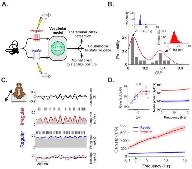
Regular and irregular otolith afferent responses to naturalistic translational self-motion stimuli.
(A) Schematic showing early vestibular pathways and recording sites. (B) Distribution of resting discharge variability as quantified by CV* for our dataset. As detailed in the Materials and methods, CV* is a normalized coefficient of variation that is used to quantify resting discharge variability independently of differences in firing rate (Goldberg et al., 1984). The distribution was clearly bimodal (Hartigan’s dip test, p=0.04). The insets show the interspike interval histograms from example regular (left, blue) and irregular (right, red) afferents with CV*=0.06 and 0.29, respectively. (C) Time varying linear head acceleration (top row) with corresponding spiking and firing rate from example irregular (second row from top) and regular (third row from top) afferents. The linear firing rate predictions for the irregular and regular afferents are shown in red and blue, respectively. The time varying residuals (i.e., difference between the actual and predicted responses) are also shown for each afferent (bottom row). (D) Population-averaged gains for regular (blue, N = 18) and irregular (red, N = 17) afferents as a function of stimulus frequency. Top left inset: Gain at 2 Hz (green arrow in bottom panel) as a function of CV*. Top right inset: Population-averaged power spectra of the residual for regular (blue) and irregular (red) afferents. The shaded bands show 1 SEM.
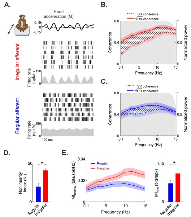
Irregular otolith afferents display greater response nonlinearity than their regular counterparts.
(A) Time-varying stimulus (top) as well as spiking- and firing-rate responses to repeated stimulus presentations, obtained from the same irregular (middle) and regular (bottom) afferents shown in Figure 1. (B) Population-averaged stimulus–response (SR, dashed red) and square root of the response–response (√RR, solid red) coherence curves for irregular afferents. (C) Population-averaged SR (dashed blue) and √RR (solid blue) coherence curves for regular afferents. (D) The population-averaged nonlinearity index values for regular (blue) and irregular (red) afferents were significantly different from one another (p=0.0002). (E) Population-averaged mutual information density curves for irregular (red) and regular (blue) afferents. Right bar chart: population-averaged mutual information rates for irregular (red) and regular (blue) afferents were significantly different from one another (p=0.04). Note that there is a one-to-one relationship between the mutual information rate density curve and √RR. Moreover, the mutual information rate is obtained by integrating the mutual information rate density over frequency, as detailed in the 'Materials and methods'. '*' indicates statistical significance at the p=0.05 level as determined using a Wilcoxon ranksum test. The shaded color bands around the curves show one SEM.
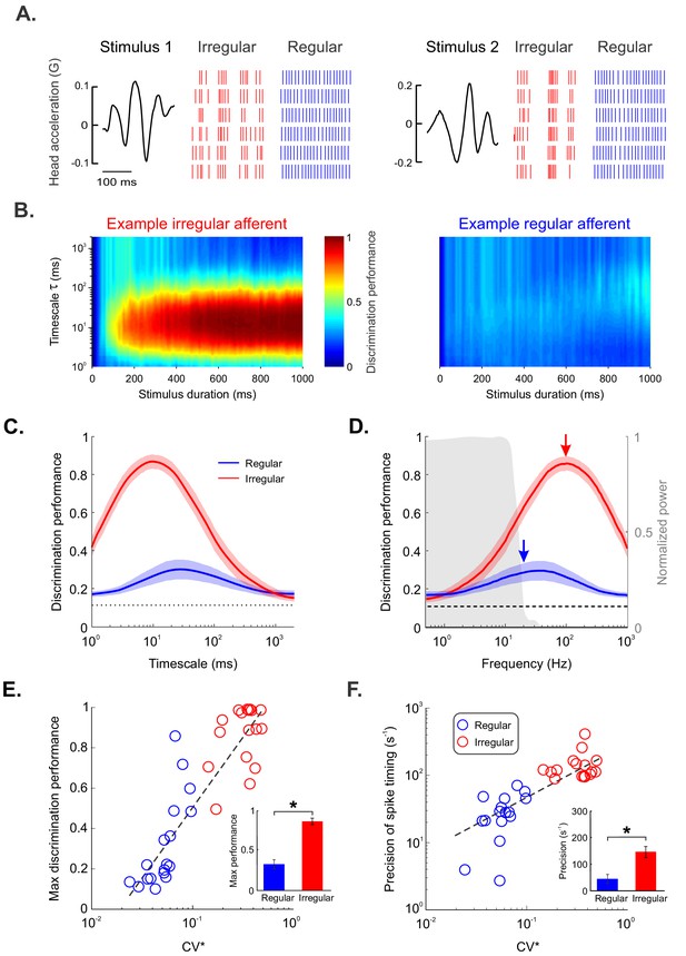
Irregular but not regular otolith afferents reliably discriminate between different stimulus waveforms through precise spike timing.
(A) Raster plots showing the spiking activities from an example irregular afferent (red) and an example regular afferent (blue) to repeated presentations of two different stimulus waveforms (left and right). (B) Discrimination performance as a function of spike-train duration and timescale τ (i.e., 1/q, see 'Materials and methods') for the example irregular afferent (left) and regular afferent (right). (C) Population-averaged discrimination performance for irregular (red) and regular (blue) afferents as a function of timescale. Chance performance is also shown (dashed line). The shaded color bands around the curves show one SEM. (D) Population-averaged discrimination performance for irregular (red) and regular (blue) afferents as a function of frequency (i.e., inverse of timescale). Chance performance (dashed line) as well as the stimulus power spectrum (shaded gray) are also shown. The shaded color bands (red and blue) around the curves show one SEM. (E, F) Discrimination performance (E) and precision of spike timing (F) as a function of baseline variability as quantified by CV* for regular (blue) and irregular (red) afferents. Afferents with higher CV* tended to display greater discrimination performance (R = 0.89, p=1.38E-12) as well as higher spike-timing precision (R = 0.71, p=4.69E-06). Insets: Population-averaged discrimination performance (E) and spike-timing precision (F) for regular (blue) and irregular (red) afferents (performance p=3.92E–06, precision p=9.26E–06). '*' indicates statistical significance at the p=0.05 level using a Wilcoxon ranksum test.
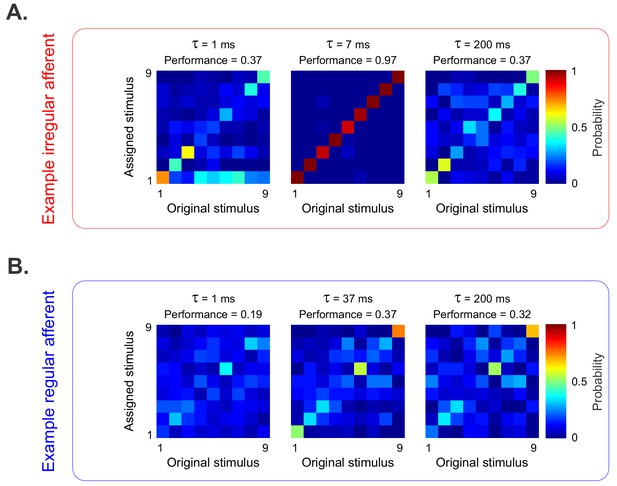
Discrimination performance is strongly linked with resting discharge variability in the otolith afferent population.
(A) Confusion matrices obtained from the example irregular afferent with the Victor-Purpura metric using timescales (1/q) of 1 ms (left), 7 ms (middle), and 200 ms (right). Element (i,j) of each matrix gives the probability of classifying a response as being elicited by stimulus i when it was in fact elicited by stimulus j. (B) Confusion matrices obtained from the example regular afferent with the Victor-Purpura metric using timescales (1/q) of 1 ms (left), 37 ms (middle), and 200 ms (right).
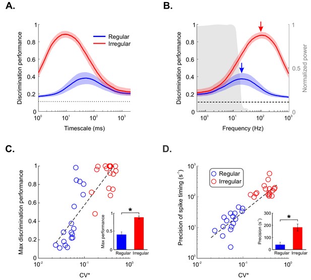
Using a different spike train metric (in this case, Van Rossum) does not affect the nature of our results.
(A) Population-averaged discrimination performance for irregular (red) and regular (blue) afferents as a function of timescale. Chance performance is also shown (dashed line). The shaded color bands around the curves show one SEM. (B) Population-averaged discrimination performance for irregular (red) and regular (blue) afferents as a function of frequency (i.e., inverse of timescale). Chance performance (dashed line) and the stimulus power spectrum (shaded great) are also shown. The shaded color bands around the curves show one SEM. (C,D) Discrimination performance (C) and precision of spike timing (D) as a function of baseline variability, as quantified by CV* for regular (blue) and irregular (red) afferents. Afferents with higher CV* tended to display greater discrimination performance (R = 0.83, p=6.27E-10) as well as higher spike-timing precision (R = 0.77, p=3.35E–8). Insets: population-averaged discrimination performance (C) and spike-timing precision (D) for regular (blue) and irregular (red) afferents were significantly different from one another (performance, p=3.95E–05; precision, p=6.49E–06). '*' indicates statistical significance at the p=0.05 level using a Wilcoxon ranksum test.
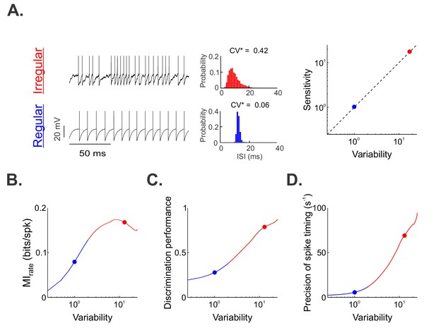
A simple mathematical model based on the leaky integrate-and-fire formalism can reproduce our experimental data by co-varying sensitivity and variability.
(A) ( Left) Example resting (i.e., in the absence of stimulation) spiking activity from our model for parameter values that reproduced data from irregular and regular afferents (CV*=0.06). (Middle) Interspike interval histograms from example irregular (top) and regular (bottom) model afferents with CV*=0.42 and 0.06, respectively. (Right) Variability as a function of sensitivity in our model. Both were co-varied such that their ratio remains unity (dashed line). (B, C, D) Mutual information rate (B), performance (C), and precision (D) as a function of variability. The blue and red dots show the values used (A) or obtained (B, C, D) for the regular and irregular afferent models, respectively. Note that because variability and sensitivity were co-varied in our model, the results obtained in (B), (C) and (D) could be similarly plotted as a function of sensitivity instead of variability.
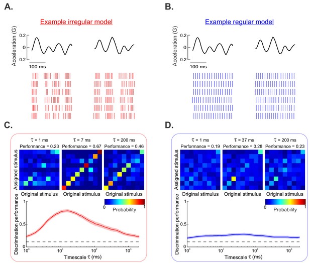
Modeling reproduces our experimental data.
(A, B) Raster plots showing the spiking responses of our irregular (A) and regular (B) afferent models to repeated presentations of two different stimulus waveforms. (C) (Top) Confusion matrices from our irregular afferent model for timescales 1 ms (left), 7 ms (middle), and 200 ms (right). (Bottom) Performance as a function of timescale for our irregular afferent model. (D) (Top) Confusion matrices from our regular afferent model for timescales 1 ms (left), 37 ms (middle), and 200 ms (right). (Bottom) Performance as a function of timescale for our regular afferent model.
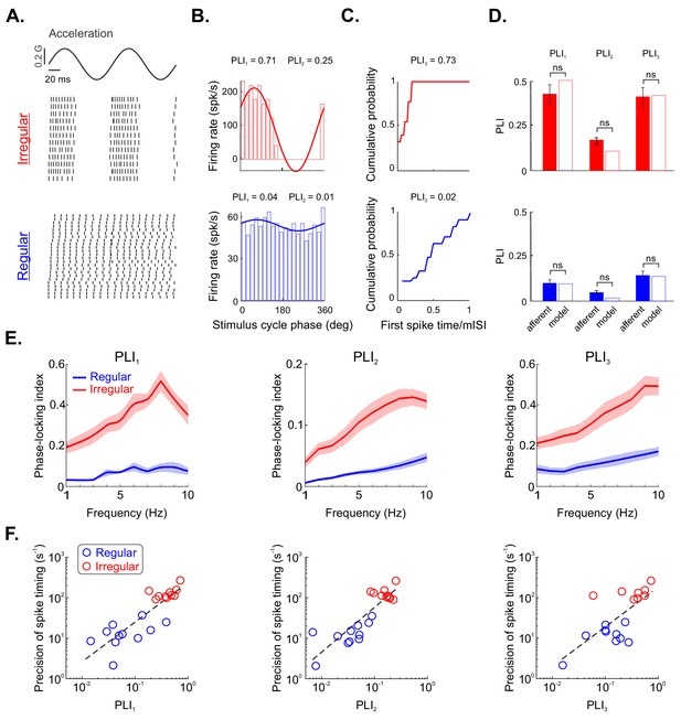
Irregular otolith afferents display greater phase locking to sinusoidal stimulation than their regular counterparts.
(A) Sinusoidal head acceleration stimulus (top) with raster plots showing the responses of example irregular (middle) and regular (bottom) afferents. (B) Plots of cycle histograms showing firing rate as a function of phase for the same example irregular (top) and regular (bottom) afferents, showing the corresponding values of PLI1 (i.e., vector strength) and PLI2 (i.e., entropy-based). (C) Plots of cumulative probability as a function of first spike time normalized by the mean interspike interval (ISI) for the same example irregular (top) and regular (bottom) afferents with the corresponding values of PLI3. (D) Population-averaged values of PLI1, PLI2, and PLI3 for irregular (top) and regular (bottom) afferents (solid). The hollow bars show the values computed from our model irregular (red) and regular (blue) afferents. Overall, no significant differences were observed (irregular PLI1, p=0.73; irregular PLI2, p=0.55; irregular PLI3, p=1; regular PLI1, p=0.83; regular PLI2, p=0.50; regular PLI3, p=1). (E) Phase locking indices PLI1 (left), PLI2 (middle), and PLI3 (right) as a function of stimulus frequency. (F) Spike-timing precision as a function of PLI1 (left), PLI2 (middle), and PLI3 (right) for regular (blue) and irregular (red) afferents. Strong positive correlations were observed in both cases (left: R = 0.84, p=1.88E–06; middle: R = 0.87, p=4.35E–07; right: R = 0.7, p=0.001).
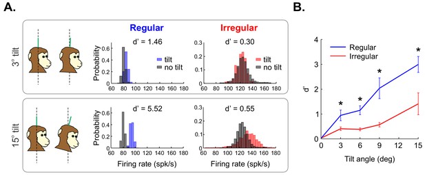
Regular otolith afferents better discriminate between different head orientations relative to gravity than do their irregular counterparts.
(A) (Top left) schematic showing the head positioned vertically (i.e., 0o, left) and at a 3o angle relative to gravity (right). (Top center) Firing rate distributions from an example regular afferent when the head is positioned at 0o (black) and at 3o (blue). (Top right) Firing rate distributions from an example irregular afferent when the head is positioned at 0o (black) and at 3o (red). Also shown are the values of discriminability d’. (Bottom) Same as top row but with a head position at a 15o angle relative to gravity. Firing rates were obtained by convolving the spike trains with a Gaussian spike-density function with standard deviation 10 ms. Firing-rate distributions were obtained using a binwidth of 4 spk/sec (as detailed in the 'Materials and methods'). (B) Population-averaged discriminability index d’ values for regular (blue) and irregular (red) otolith afferents as a function of head orientation angle. '*' indicates statistical significance at the p=0.05 level using a Wilcoxon ranksum test.
Additional files
-
Transparent reporting form
- https://doi.org/10.7554/eLife.45573.011


