Neural ensemble dynamics in dorsal motor cortex during speech in people with paralysis
- Stanford University, United States
- Case Western Reserve University, United States
- Louis Stokes Cleveland Department of Veterans Affairs Medical Center, United States
- University Hospitals Cleveland Medical Center, United States
- Providence VA Medical Center, United States
- Massachusetts General Hospital, Harvard Medical School, United States
- Brown University, United States
- Howard Hughes Medical Institute, Stanford University, United States
Figures
Figure 1 with 5 supplements

Speech-related neuronal spiking activity in dorsal motor cortex.
(A) Participants heard a syllable or word prompt played from a computer speaker and were instructed to speak it back after hearing a go cue. Motor cortical signals and audio were simultaneously recorded during the task. The timeline shows example audio data recorded during one trial. (B) Participants’ MRI-derived brain anatomy. Blue squares mark the locations of the two chronic 96-electrode arrays. Insets show electrode locations, with shading indicating the number of different syllables for which that electrode recorded significantly modulated firing rates (darker shading = more syllables). Non-functioning electrodes are shown as smaller dots. CS is central sulcus. (C) Raster plot showing spike times of an example neuron across multiple trials of participant T5 speaking nine different syllables, or silence. Data are aligned to the prompt, the go cue, and acoustic onset (AO). (D) Trial-averaged firing rates (mean ± s.e.) for the same neuron and two others. Insets show these neurons’ action potential waveforms (mean ± s.d.). The electrodes where these neurons were recorded are circled in the panel B insets using colors corresponding to these waveforms. (E) Time course of overall neural modulation for each syllable after hearing the prompt (left alignment) and when speaking (right alignment). Population neural distances between the spoken and silent conditions were calculated from TCs using an unbiased measurement of firing rate vector differences (see Methods). This metric yields signed values near zero when population firing rates are essentially the same between conditions. Firing rate changes were significantly greater (p < 0.01, sign-rank test) during speech production (comparison epoch shown by the black window after Go) compared to after hearing the prompt (gray window after Prompt). Each syllable’s mean modulation across the comparison epoch is shown with the corresponding color’s horizontal tick to the right of the plot. The vertical scale is the same across participants, revealing the larger speech-related modulation in T5’s recordings.
Figure 1—figure supplement 1
Prompted speaking tasks behavior.
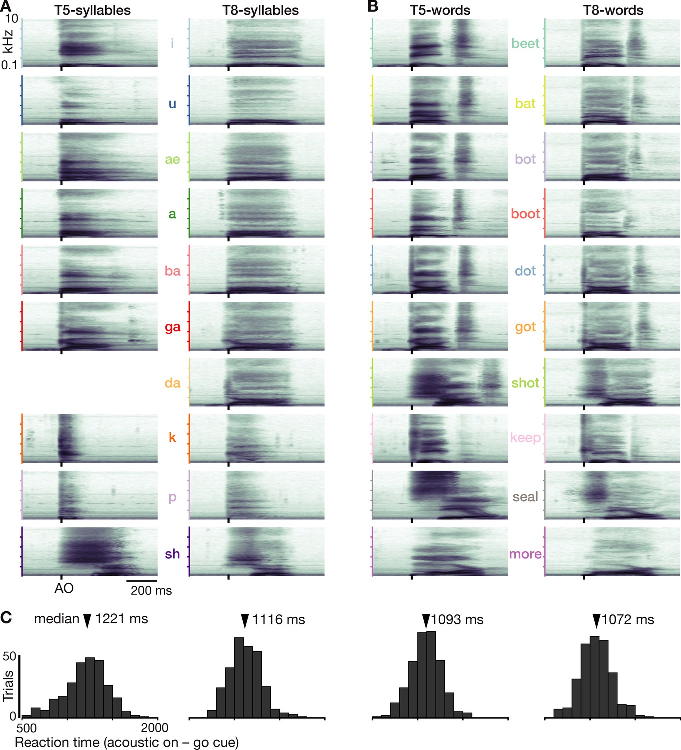
(A) Acoustic spectrograms for the participants’ spoken syllables. Power was averaged over all analyzed trials. Note that da is missing for T5 because he usually misheard this cue as ga or ba. (B) Same as panel A but for the words datasets. (C) Reaction time distributions for each dataset.
Figure 1—figure supplement 2
Example threshold crossing spike rates.
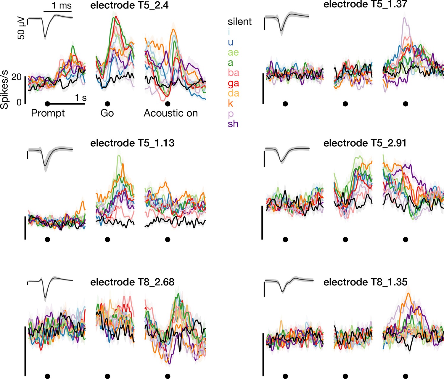
The left column shows –4.5 × root mean square voltage threshold crossing firing rates during the syllables task, recorded on the electrodes from which the single neuron spikes in Figure 1D were spike sorted. The right column shows three additional example electrodes’ firing rates. Insets shows the unsorted threshold crossing spike waveforms.
Figure 1—figure supplement 3
Neural activity while speaking short words.
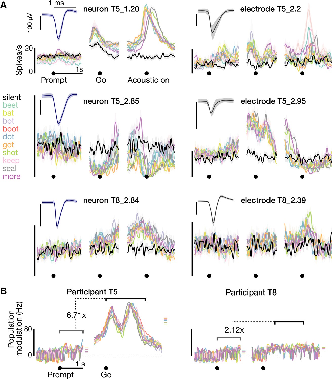
(A) Firing rates during speaking of short words for three example neurons (blue spike waveform insets) and three example electrodes’ −4.5 × RMS threshold crossing spikes (gray waveform insets). Data are presented similarly to Figure 1D and are from the T5-words and T8-words datasets. (B) Firing rate differences compared to the silent condition across the population of threshold crossings, presented as in Figure 1E. The ensemble modulation was significantly greater when speaking words compared to when hearing the prompts (p<0.01, sign-rank test).
Figure 1—figure supplement 4
Neural correlates of spoken syllables are not spatially segregated in dorsal motor cortex.
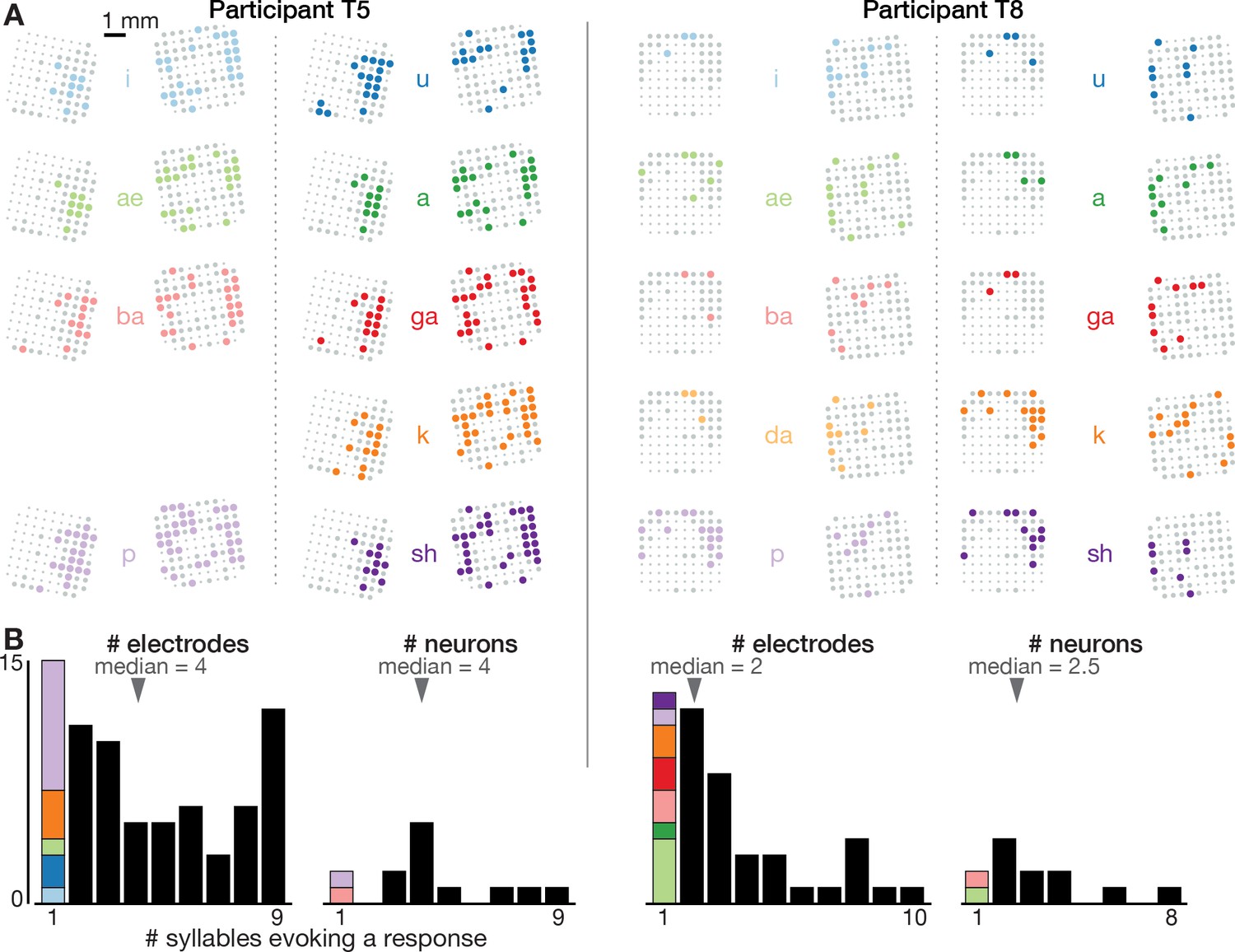
(A) Electrode array maps similar to Figure 1B insets are shown for each syllable separately to reveal where modulation was observed during production of that sound. Electrodes where the TCs firing rate changed significantly during speech, as compared to the silent condition, are shown as colored circles. Non-modulating electrodes are shown as larger gray circles, and non-functioning electrodes are shown as smaller dots. Adding up how many different syllables each electrode’s activity modulates to yields the summary insets shown in Figure 1B. These plots reveal that electrodes were not segregated into distinct cortical areas based on which syllables they modulated to. (B) Histograms showing the distribution of how many different syllables evoke a significant firing rate change for electrode TCs (each participant’s left plot) and sorted single neurons (right plot). The first bar in each plot, which corresponds to electrodes or neurons whose activity only changed when speaking one syllable, is further divided based on which syllable this modulation was specific to (same color scheme as in panel A). This reveals two things. First, single neurons or TCs (which may capture small numbers of nearby neurons) were typically not narrowly tuned to one sound. Second, there was not one specific syllable whose neural correlates were consistently observed on separate electrodes/neurons from the rest of the syllables.
Figure 1—figure supplement 5
Neural activity shows phonetic structure.
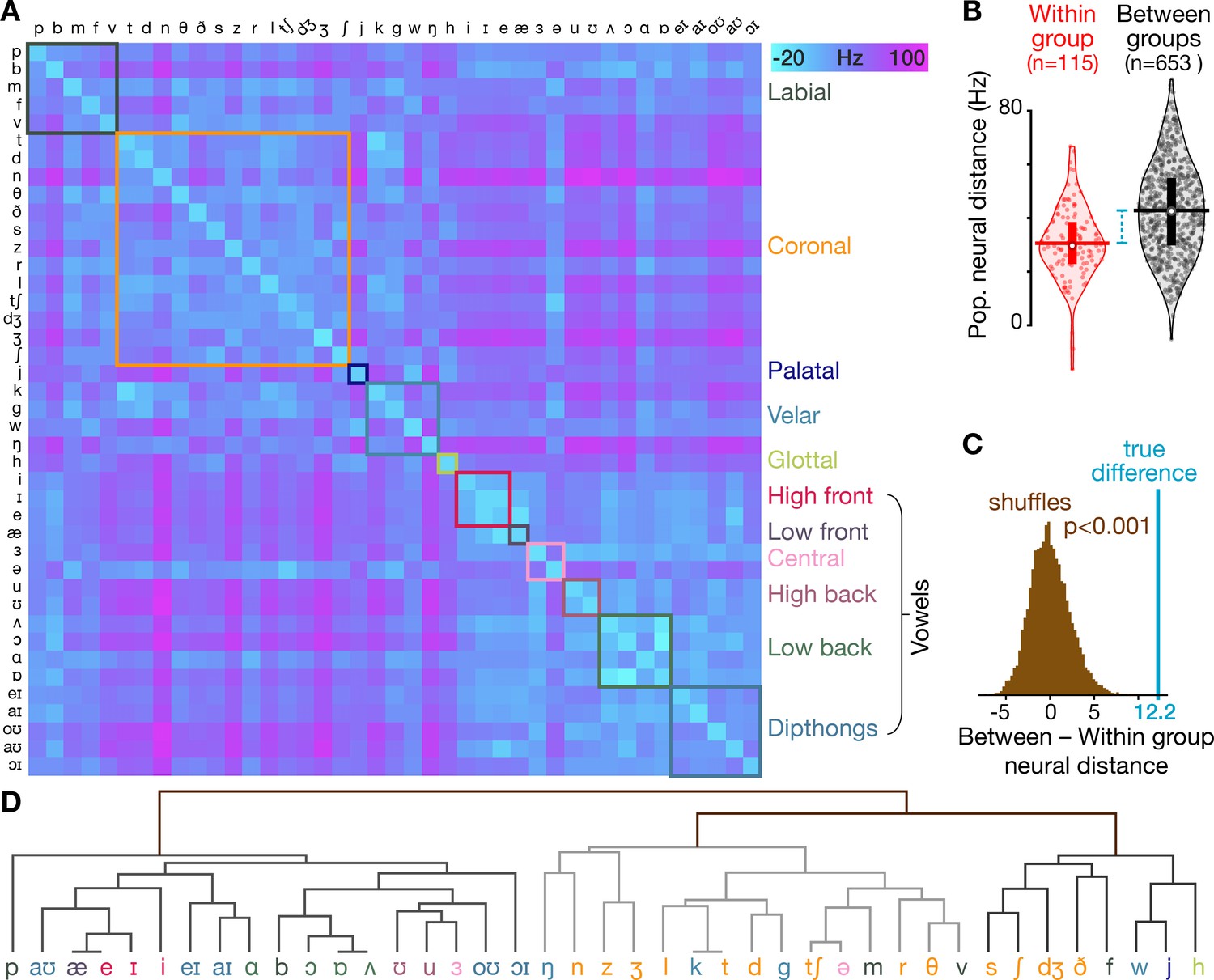
(A) The T5-phonemes dataset consists of the participant speaking 420 unique words which together sampled 41 American English phonemes. We constructed firing rate vectors for each phoneme using a 150 ms window centered on the phoneme start (one element per electrode), averaged across every instance of that phoneme. This dissimilarity matrix shows the difference between each pair of phonemes’ firing rate vectors, calculated using the same neural distance method as in Figure 1E. The matrix is symmetrical across the diagonal. Diagonal elements (i.e. within-phoneme distances) were constructed by comparing split halves of each phoneme’s instances. The phonemes are ordered by place of articulation grouping (each group is outlined with a box of different color). (B) Violin plots showing all neural distances from panel A divided based on whether the two compared phonemes are in the same place of articulation group (‘Within group’, red) or whether the two phonemes are from different place of articulation groups (‘Between groups’, black). Center circles show each distribution’s median, vertical bars show 25th to 75th percentiles, and horizontal bars shows distribution means. The mean neural distance across all Within group pairs was 30.6 Hz, while the mean across all Between group pairs was 42.8 Hz (difference = 12.2 Hz). (C) The difference in between-group versus within-group neural distances from panel B, marked with the blue line, far exceeds the distribution of shuffled distances (brown) in which the same summary statistic was computed 10,000 times after randomly permuting the neural distance matrix rows and columns. These shuffles provide a null control in which the relationship between phoneme pairs’ neural activity differences and these phonemes’ place of articulation groupings are scrambled. (D) A hierarchical clustering dendrogram based on phonemes’ neural population distances from panel A. At the bottom level, each phoneme is placed next to the (other) phoneme with the most similar neural population activity. Successive levels combine nearest phoneme clusters. By grouping phonemes based solely on their neural similarities (rather than one specific trait like place of articulation, indicated here with the same colors as in the panel A groupings), this dendrogram provides a complementary view that highlights that many neural nearest neighbors are phonetically similar (e.g. /d/ and /g/ stop-plosives, /θ/ and /v/ fricatives, /ŋ/ and /n/ nasals) and that related phonemes form larger clusters, such as the left-most major branch of mostly vowels or the sibilant cluster /s/, /ʃ/, and /dʒ/. At the same time, there are some phonemes that appear out of place, such as plosive consonant /b/ appearing between vowels /ɑ/ and /ɔ/ (we speculate this could reflect neural correlates of co-articulation from the vowels that frequently followed the brief /b/ sound).
Figure 2 with 3 supplements
The same motor cortical population is also active during non-speaking orofacial movements.
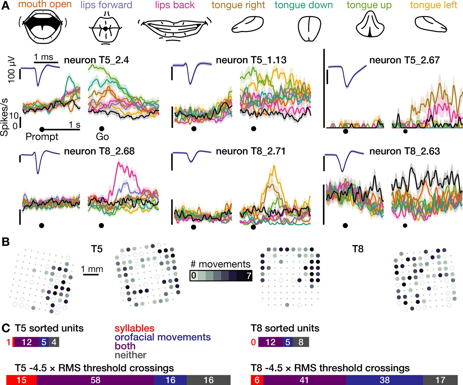
(A) Both participants performed an orofacial movement task during the same research session as their syllables speaking task. Examples of single neuron firing rates during seven different orofacial movements are plotted in colors corresponding to the movements in the illustrated legend above. The ‘stay still’ condition is plotted in black. The same three example neurons from Figure 1D are included here. The other three neurons were chosen to illustrate a variety of observed response patterns. (B) Electrode array maps indicating the number of different orofacial movements for which a given electrode’s −4.5 × RMS threshold crossing rates differed significantly from the stay still condition. Data are presented similarly to the Figure 1B insets. Firing rates on most functioning electrodes modulated for multiple orofacial movements. See Figure 2—figure supplement 1 for individual movements’ electrode response maps. (C) Breakdown of how many neurons’ (top) and electrodes’ TCs (bottom) exhibited firing rate modulation during speaking syllables only (red), non-speaking orofacial movements only (blue), both behaviors (purple), or neither behavior (gray). A unit or electrode was deemed to modulate during a behavior if its firing rate differed significantly from silence/staying still for at least one syllable/movement.
Figure 2—figure supplement 1
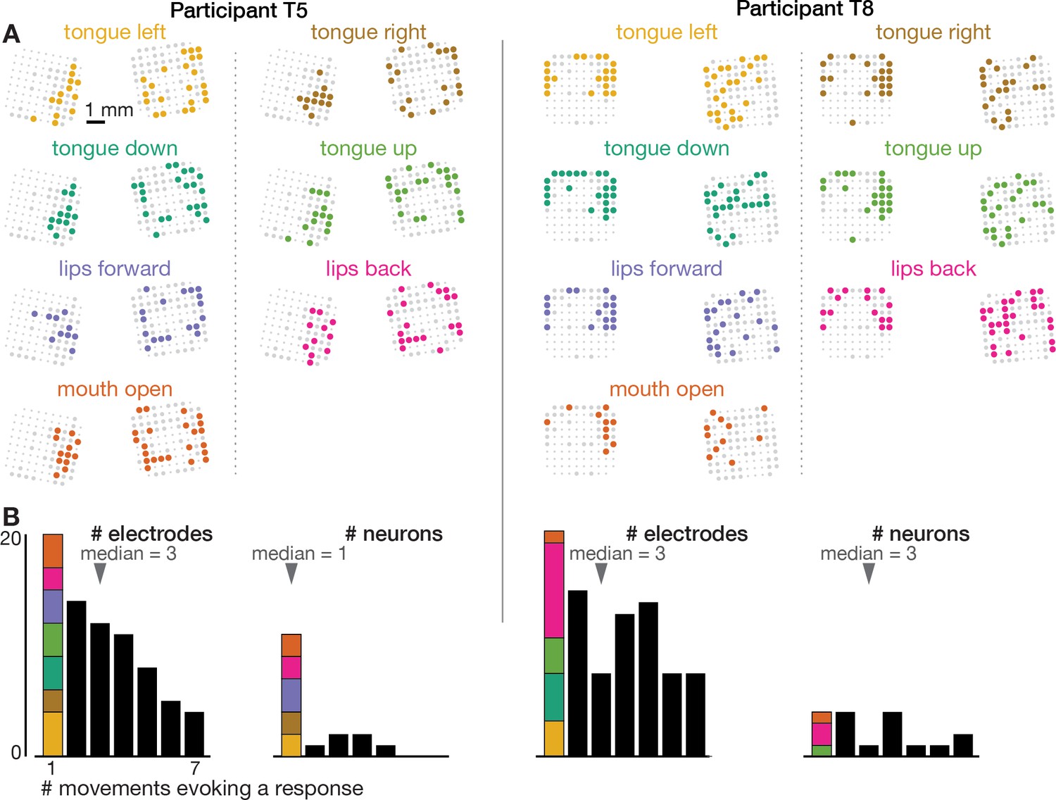
Neural correlates of orofacial movements are not spatially segregated in dorsal motor cortex.
The orofacial movements data were analyzed and are presented like the speaking data in Figure 1—figure supplement 4.
Figure 2—figure supplement 2
Dorsal motor cortex correlates of breathing.
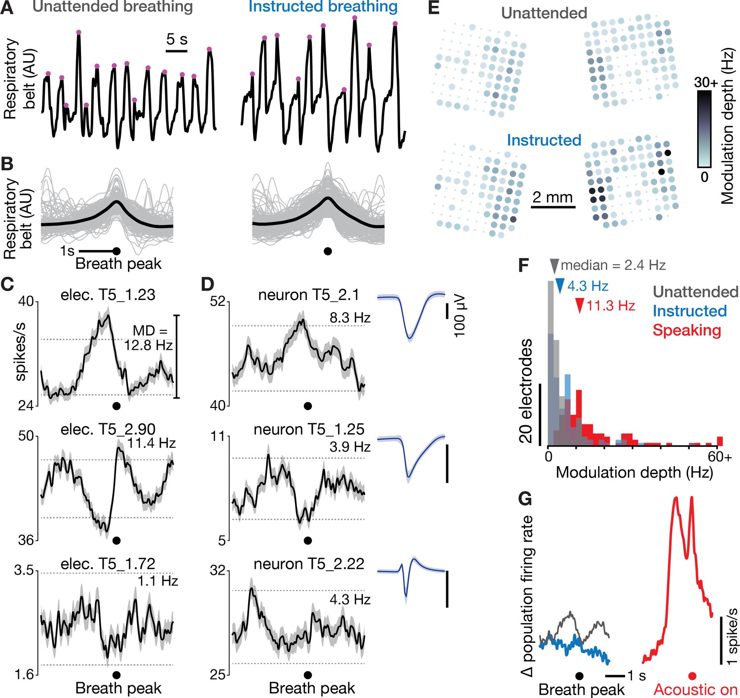
(A) We recorded neural data and a breathing proxy (the stretch of a belt wrapped around participant T5’s abdomen) while he performed a BCI cursor task or sat idly (‘unattended’ breathing condition, left) or intentionally breathed in and out based on on-screen instructions (‘instructed’, right). Example continuous breath belt measurements from this T5-breathing dataset are shown. Violet dots mark the identified breath peak times. (B) Gray traces show example respiratory belt measurements for 200 unattended (left) and instructed (right) breaths, aligned to the breath peak. The means of all 727 unattended and 275 instructed breaths are shown in black. (C) Breath-aligned firing rates for three example electrodes’ TCs (mean ± s.e.m) during unattended breathing. Breath-related modulation depth was calculated as the peak-to-trough firing rate difference. Horizontal dashed lines show the p=0.01 modulation depths for a shuffle control in which breath peak times were chosen at random. Significantly greater breath-related modulation in either the unattended or instructed condition was observed on 71 out of 121 electrodes. (D) Breath-aligned firing rates were also calculated for sortable SUA, whose spike waveform snippets are shown as in Figure 1D. Firing rates of three example neurons with large waveforms are shown during unattended breathing. Overall, 17 out of 19 sorted units had significant modulation in either the unattended or instructed condition. This argues against the breath-related modulation being an artifact of breath-related electrode array micromotion causing a change in TCs firing rates by bringing additional units in or out of recording range. (E) Unattended (top) and instructed (bottom) breath-related modulation depth for each functioning electrode’s TCs, presented as in Figure 1B. Two extrema values exceeded the 30 Hz color range maximum. (F) Histograms of modulation depths during unattended breathing (gray), instructed breathing (blue), and speaking-related modulation depths (red) for all functioning electrodes in the T5-breathing and T5-syllables datasets, respectively. Two outlier datums are grouped in a > 60 Hz bin. Dorsal motor cortical modulation was greater for speaking than breathing (all three distributions significantly differed from one another, p<0.001, rank-sum tests). (G) Mean population firing rates (averaged across all functioning electrodes) are shown during unattended (gray) and instructed (blue) breathing, aligned to breath peak, and during speaking (red), aligned to acoustic onset. The vertical offsets of the breathing traces have been bottom-aligned to the speaking trace to facilitate comparison. Note that the mean population rate can obscure counter-acting firing rate increases and decreases across electrodes; panel F provides a complementary description capturing both rate increases and decreases.
Figure 2—figure supplement 3
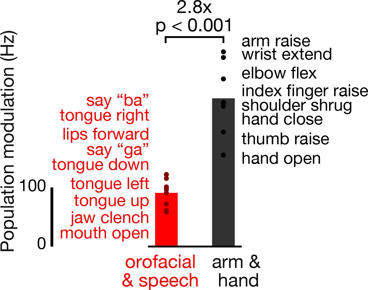
Dorsal motor cortex modulates more strongly during attempted arm and hand movements than orofacial movements and speaking.
Participant T5 performed a variety of instructed movements. We compared neural activity when attempting orofacial and speech production movements (red), versus when attempting arm and hand movements (black). Note that T5, who has tetraplegia, was able to actualize all the orofacial and speech movements, but not all the arm and hand movements. Each point corresponds to the mean TCs firing rate modulation for a single instructed movement (movements are listed in the order corresponding to their points’ vertical coordinates) in the T5-comparisons dataset. Modulation strength is calculated by taking the firing rate vector neural distance (like in Figure 1E) between when T5 attempted/performed the instructed movement and otherwise similar trials where the instruction was to ‘do nothing’. Bars show the mean modulation across all the movements in each grouping. A rank-sum test was used to compare the distributions of orofacial and speech and arm and hand modulations.
Figure 3
Speech can be decoded from intracortical activity.
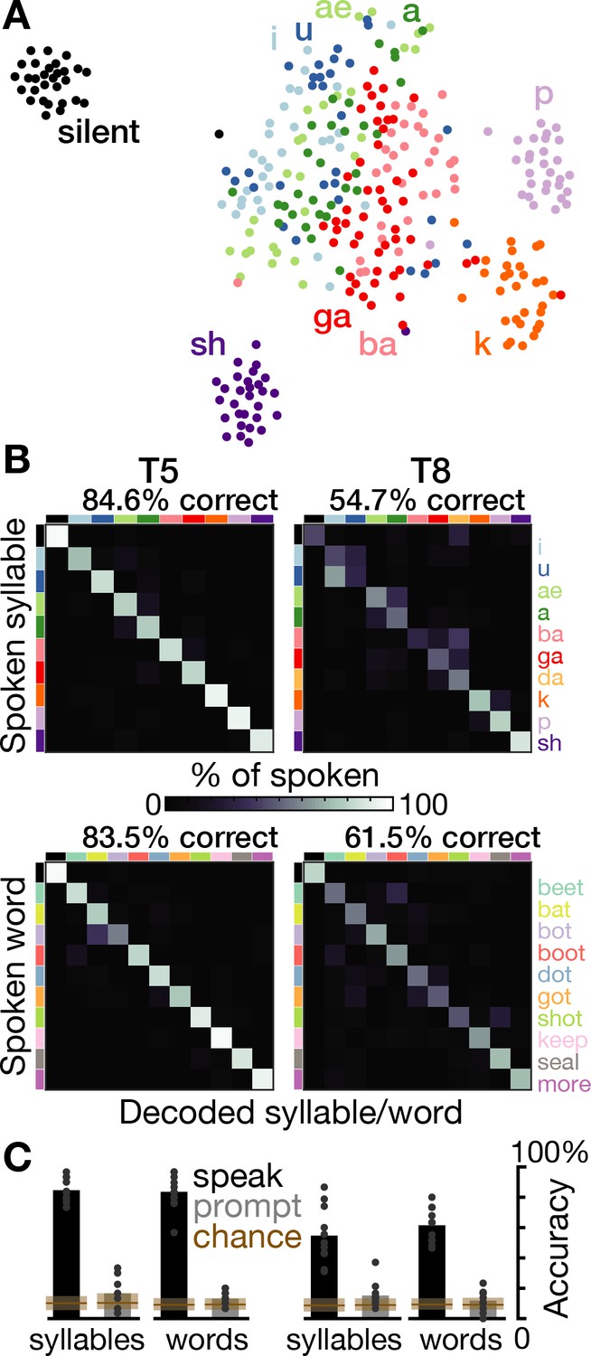
(A) To quantify the speech-related information in the neural population activity, we constructed a feature vector for each trial consisting of each electrode’s spike count and HLFP power in ten 100 ms bins centered on AO. For visualization, two-dimensional t-SNE projections of this feature vector are shown for all trials of the T5-syllables dataset. Each point corresponds to one trial. Even in this two-dimensional view of the underlying high-dimensional neural data, different syllables’ trials are discriminable and phonetically similar sounds’ clusters are closer together. (B) The high-dimensional neural feature vectors were classified using a multiclass SVM. Confusion matrices are shown for each participant’s leave-one-trial-out classification when speaking syllables (top row) and words (bottom row). Each matrix element shows the percentage of trials of the corresponding row’s sound that were classified as the sound of the corresponding column. Diagonal elements show correct classifications. (C) Bar heights show overall classification accuracies for decoding neural activity during speech (black bars, summarizing panel B) and decoding neural activity following the audio prompt (gray bars). Each small point corresponds to the accuracy for one class (silence, syllable, or word). Brown boxes show the range of chance performance: each box’s bottom/center/top correspond to minimum/mean/maximum overall classification accuracy for shuffled labels.
Figure 4 with 2 supplements
A condition-invariant signal during speech initiation.
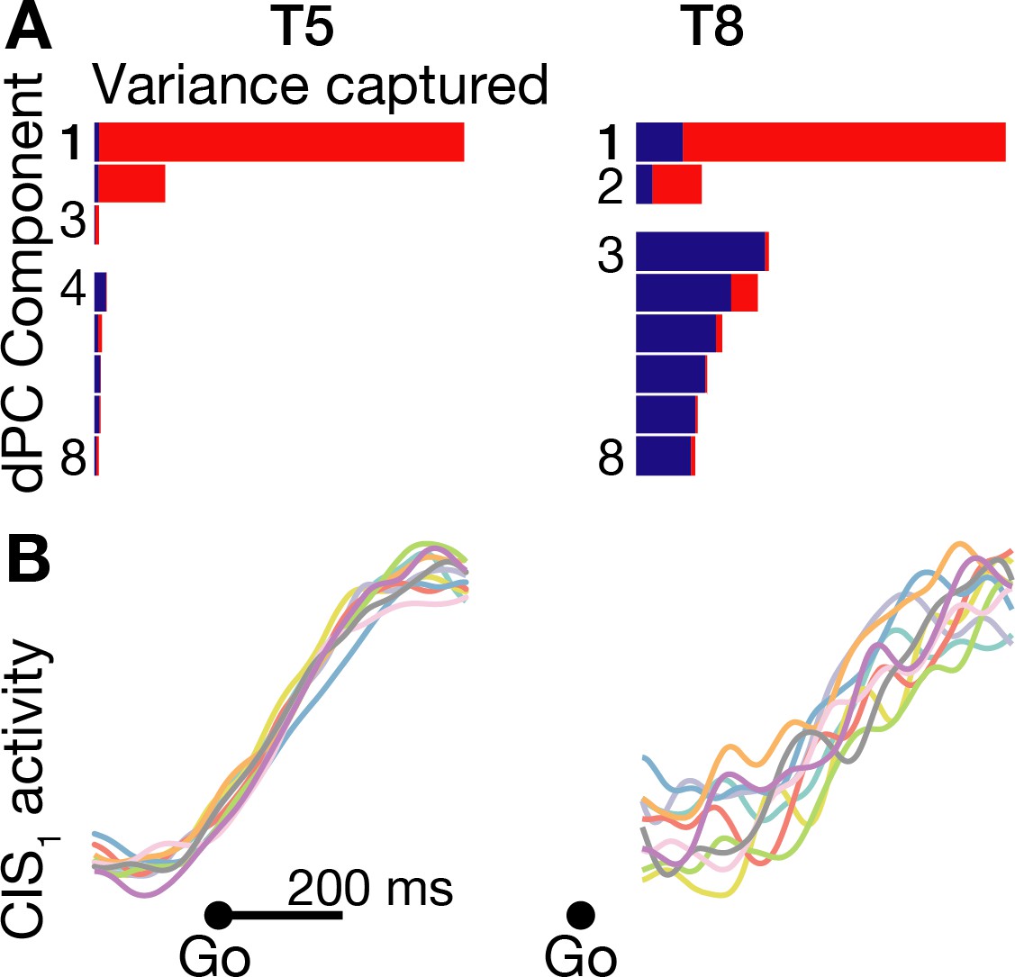
(A) A large component of neural population activity during speech initiation is a condition-invariant (CI) neural state change. Firing rates from 200 ms before to 400 ms after the go cue (participant T5) and 100 ms to 700 ms after the go cue (T8) were decomposed into dPCA components like in Kaufman et al. (2016). Each bar shows the relative variance captured by each dPCA component, which consists of both CI variance (red) and condition-dependent (CD) variance (blue). These eight dPCs captured 45.1% (T5-words) and 8.4% (T8-words) of the overall neural variance, which includes non-task related variability (‘noise’). (B) Neural population activity during speech initiation was projected onto the first dPC dimension; this ‘CIS1’ is the first component from panel A. Traces show the trial-averaged CIS1 activity when speaking different words, denoted by the same colors as in Figure 3B.
Figure 4—figure supplement 1
Further details of neural population dynamics analyses and additional datasets.
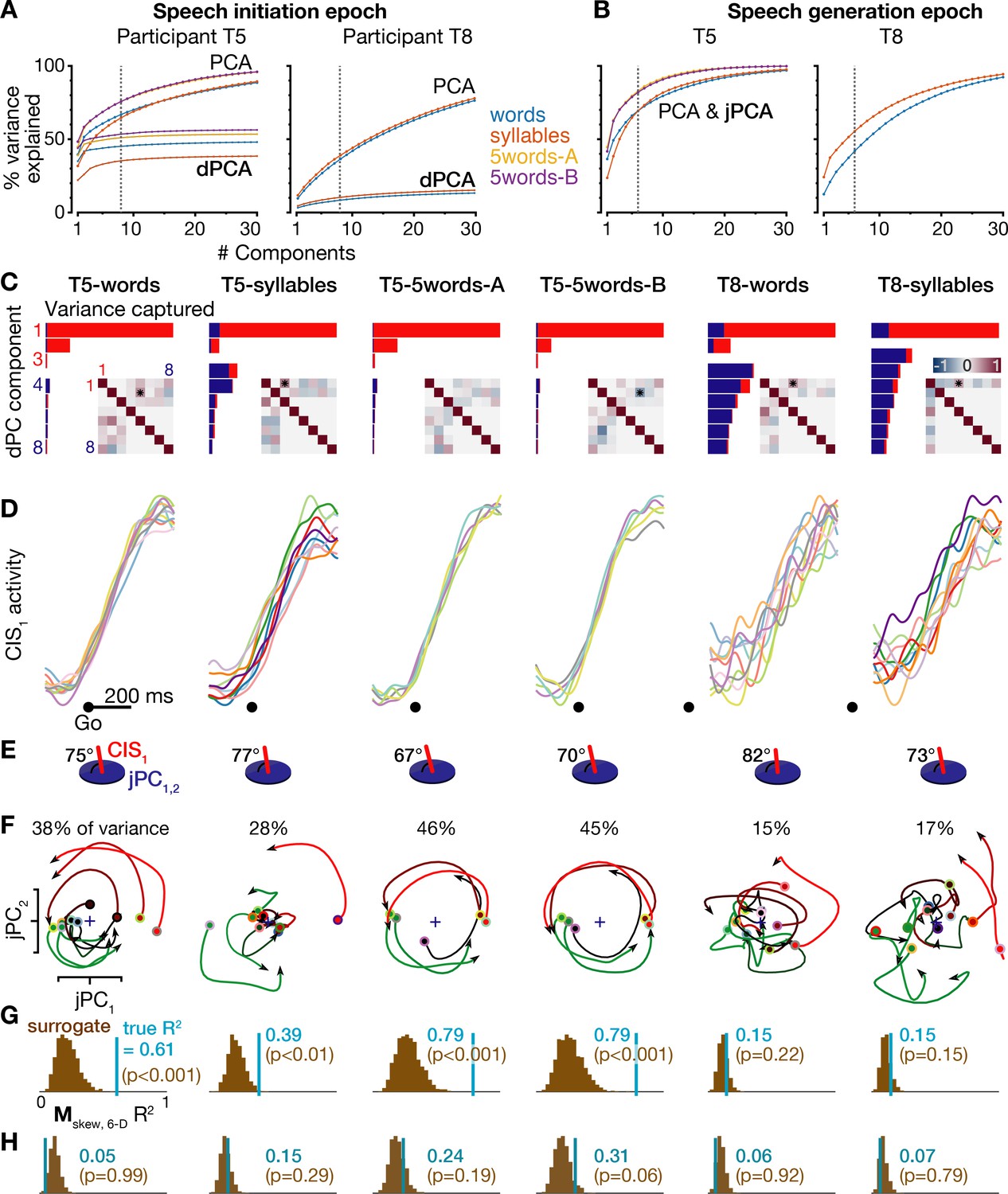
(A) Cumulative trial-averaged firing rate variance explained during each dataset’s speech initiation epoch as a function of the number of PCA dimensions (top set of curves) and dPCA dimensions (bottom set of curves) used to reduce the dimensionality of the data. The dotted lines mark the eight dimensions used for dPCA in the condition-invariant signal analyses for panels C-E and in Figure 4. In addition to the T5-words and T8-words datasets (blue curves) shown in Figure 4, this figure also shows results from the T5-syllables and T8-syllables datasets (orange curves) as well as the T5-5words-A and T5-5words-B replication datasets (gold and purple curves). (B) Cumulative trial-averaged firing rate variance explained during all six datasets’ speech generation epochs. The dotted lines mark the six dimensions used for jPCA in the rotatory dynamics analyses for panels E-H and Figure 5. PCA and jPCA curves are one and the same because jPCA operates within the neural subspace found using PCA. (C) Firing rates during the speech initiation epoch of each dataset were decomposed into dPCA components like in Figure 4A. The additional inset matrices quantify the relationships between dPC components as in Kobak et al. (2016): each element of the upper triangle shows the dot product between the corresponding row’s and column’s demixed principal axes (i.e. the dPCA encoder dimensions), while the bottom triangle shows the correlations between the corresponding row’s and column’s demixed principal components (i.e. the neural data projected onto this row’s and column’s demixed principal decoder axes). More red or blue upper triangle elements denote that this pair of neural dimensions are less orthogonal, while more red or blue lower triangle elements denote that this pair of components (summarized population firing rates) have a similar time course. Stars denote pairs of dimensions that are significantly non-orthogonal at p<0.01 (Kendall correlation). (D) Neural population activity projected onto the first dPC dimension, shown as in Figure 4B for all six datasets. (E) The subspace angle between the CIS1 dimension from panels C,D and the top jPC plane from panel F, for each dataset. Across all six datasets, the CIS1 was not significantly non-orthogonal to any of the six jPC dimensions (p>0.01, Kendall correlation) except for the angle between CIS1 and jPC5 in the T5-words dataset (70.5°, p<0.01). (F) Neural population activity for each speaking condition was projected into the top jPCA plane as in Figure 5A, for all six datasets. (G) The same statistical significance testing from Figure 5B was applied to all datasets to measure how well a rotatory dynamical system fit ensemble neural activity. (H) Rotatory neural population dynamics were not observed when the same jPCA analysis was applied on each dataset’s neural activity from 100 to 350 ms after the audio prompt. Rotatory dynamics goodness of fits are presented as in the previous panel.
Figure 4—figure supplement 2
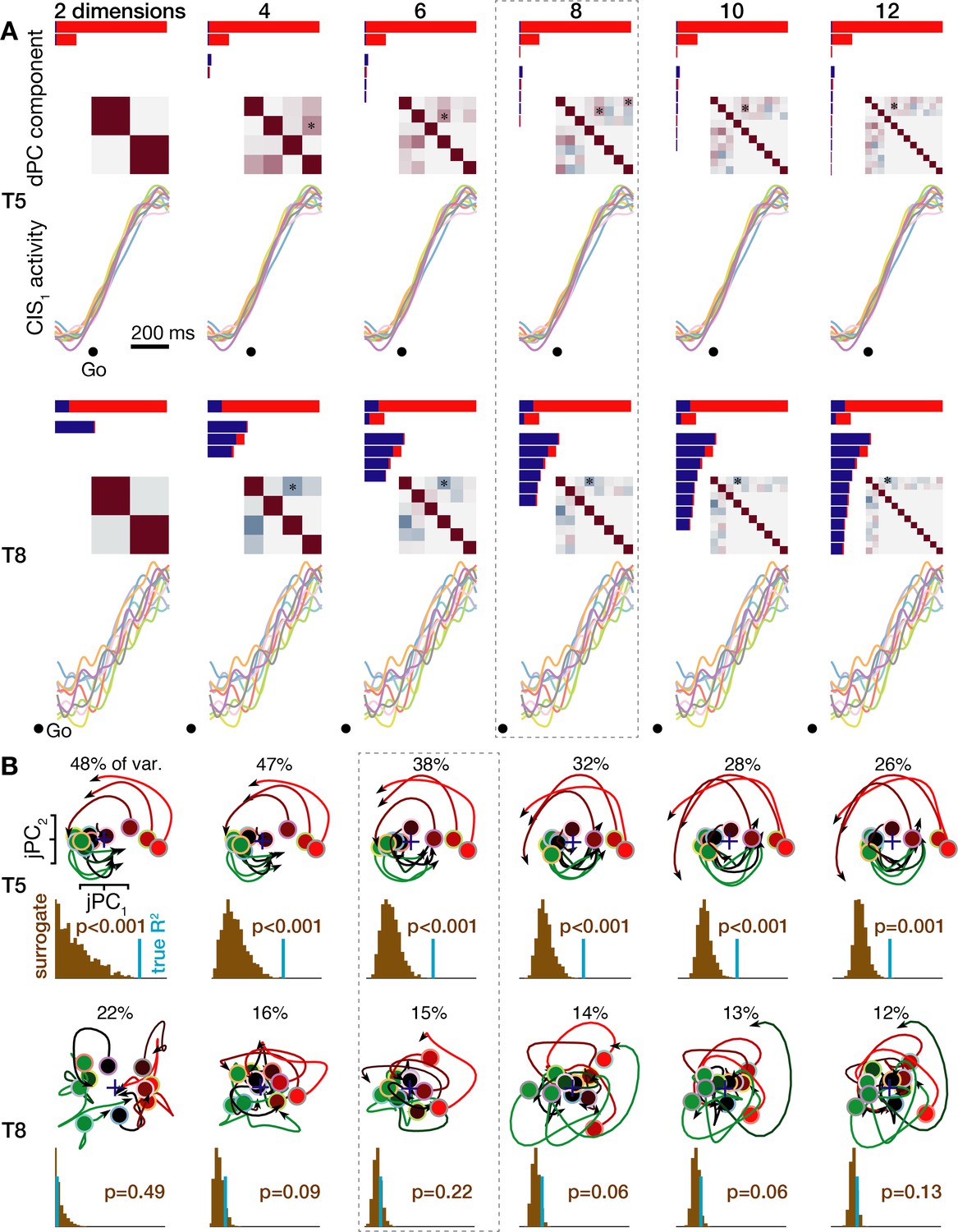
Neural population dynamics when viewed across a range of reduced dimensionalities.
(A) Condition-invariant neural population dynamics during speech initiation are summarized as in Figure 4 for the T5-words (top) and T8-words (bottom) datasets, but now varying the number of dPCA components used for dimensionality reduction. The eight dPCs results shown in Figure 4 and Figure 4—figure supplement 1 are outlined with a dashed gray box. (B) Rotatory neural population dynamics during speaking are summarized as in Figure 5 for the T5-words (top) and T8-words (bottom) datasets, but now varying the number of principal components used for the initial dimensionality reduction (after which the jPCA algorithm looks for rotatory planes). The six PCs results shown in Figure 5 and Figure 4—figure supplement 1 are outlined.
Figure 5
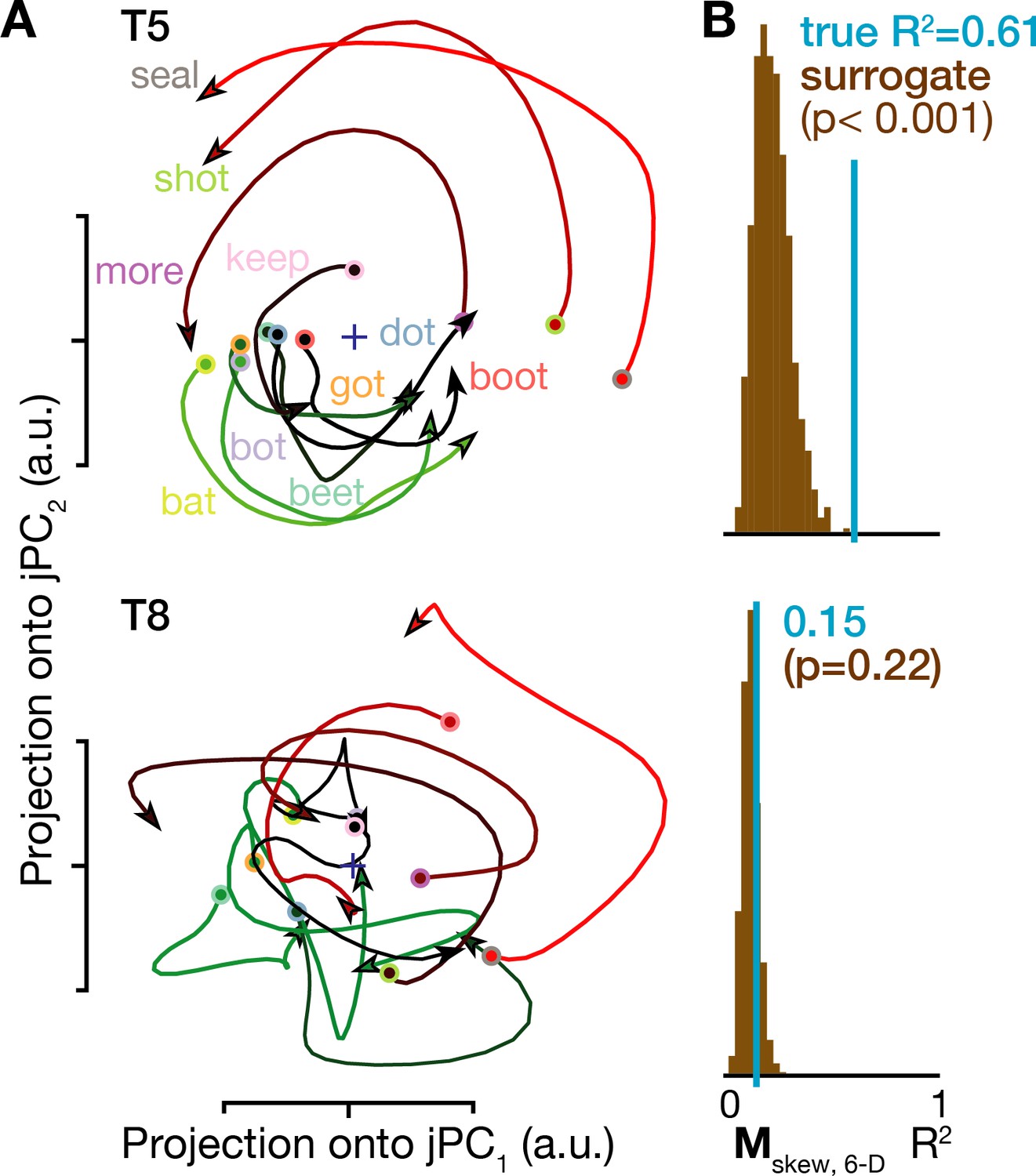
Rotatory neural population dynamics during speech.
(A) The top six PCs of the trial-averaged firing rates from 150 ms before to 100 ms after acoustic onset in the T5-words and T8-words datasets were projected onto the first jPCA plane like in Churchland et al. (2012). This plane captures 38% of T5’s overall population firing rates variance, and rotatory dynamics fit the moment-by-moment neural state change with R2 = 0.81 in this plane and 0.61 in the top 6 PCs. In T8, this plane captures 15% of neural variance, with a rotatory dynamics R2 of only 0.32 in this plane and 0.15 in the top six PCs. (B) Statistical significance testing of rotatory neural dynamics during speaking. The blue vertical line shows the goodness of fit of explaining the evolution in the top six PC’s neural state from moment to moment using a rotatory dynamical system. The brown histograms show the distributions of this same measurement for 1000 neural population control surrogate datasets generated using the tensor maximum entropy method of Elsayed and Cunningham (2017). These shuffled datasets serve as null hypothesis distributions that have the same primary statistical structure (mean and covariance) as the original data across time, electrodes, and word conditions, but not the same higher order statistical structure (e.g. low-dimensional rotatory dynamics).
Videos
Video 1
Example audio and neural data from eleven contiguous trials of the prompted syllables speaking task.
The audio track was recorded during the task and digitized alongside the neural data; it starts with the two beeps indicating trial start, after which the syllable prompt was played from computer speakers, followed by the go cue clicks, and finally the participant speaking the syllable. The video shows the concurrent −4.5 × RMS threshold crossing spikes rate on each electrode. Each circle corresponds to one electrode, with their spatial layout corresponding to electrodes’ locations in motor cortex as in the Figure 1B inset. Each electrode’s moment-by-moment color and size represent its firing rate (soft-normalized with a 10 Hz offset, smoothed with a 50 ms s.d. Gaussian kernel). The color map goes from pink (minimum rate across electrodes) to yellow (maximum rate), while size varies from small (minimum rate) to large (maximum rate). Non-functioning electrodes are shown as small gray dots. To assist the viewer in perceiving the gestalt of the population activity, a larger central disk shows the mean firing rate across all functioning electrodes, without soft-normalization. Data are from the T5-syllables dataset, trial set #23.
Video 2
The progression of neural population activity during the prompted words task is summarized with dimensionality reduction chosen to highlight the condition-invariant ‘kick’ after the go cue, followed by rotatory population dynamics.
T5-words dataset neural state space trajectories are shown from 2.5 s before go cue to 2.0 s after go. Each trajectory corresponds to one word condition’s trial-averaged firing rates, aligned to the go cue. The neural states are projected into a three-dimensional space consisting of the CIS1 dimension (as in Figure 4) and the first two jPC dimensions (similar to Figure 5, except that for this visualization we enforced that the jPC plane be orthogonal to the CIS1; see Materials and methods). The trajectories change color based on the task epoch: gray is before the audio prompt, blue is after the prompt, and then red-to-green is after the go cue, with conditions ordered as in Figure 5.
Video 3
The same neural trajectories as Video 2, but aligned to acoustic on (AO), are shown from 3.5 s before AO to 1.0 s after AO.
Additional files
-
Source data 1
Breathing data.
- https://cdn.elifesciences.org/articles/46015/elife-46015-data1-v2.zip
-
Source data 2
Classification data.
- https://cdn.elifesciences.org/articles/46015/elife-46015-data2-v2.zip
-
Source data 3
Dynamics data.
- https://cdn.elifesciences.org/articles/46015/elife-46015-data3-v2.zip
-
Source data 4
PSTHs sorted units data.
- https://cdn.elifesciences.org/articles/46015/elife-46015-data4-v2.zip
-
Source data 5
Syllables PSTHS TCs data.
- https://cdn.elifesciences.org/articles/46015/elife-46015-data5-v2.zip
-
Source data 6
Tuning and behavior data.
- https://cdn.elifesciences.org/articles/46015/elife-46015-data6-v2.zip
-
Source data 7
Video go aligned data.
- https://cdn.elifesciences.org/articles/46015/elife-46015-data7-v2.zip
-
Source data 8
Video and dynamics speak aligned data.
- https://cdn.elifesciences.org/articles/46015/elife-46015-data8-v2.zip
-
Source data 9
Words PSTHs TCs data.
- https://cdn.elifesciences.org/articles/46015/elife-46015-data9-v2.zip
-
Transparent reporting form
- https://cdn.elifesciences.org/articles/46015/elife-46015-transrepform-v2.docx
Download links
A two-part list of links to download the article, or parts of the article, in various formats.
Downloads (link to download the article as PDF)
Open citations (links to open the citations from this article in various online reference manager services)
Cite this article (links to download the citations from this article in formats compatible with various reference manager tools)
Neural ensemble dynamics in dorsal motor cortex during speech in people with paralysis
eLife 8:e46015.
https://doi.org/10.7554/eLife.46015


