Motor cortex signals for each arm are mixed across hemispheres and neurons yet partitioned within the population response
- Columbia University, United States
Figures
Figure 1
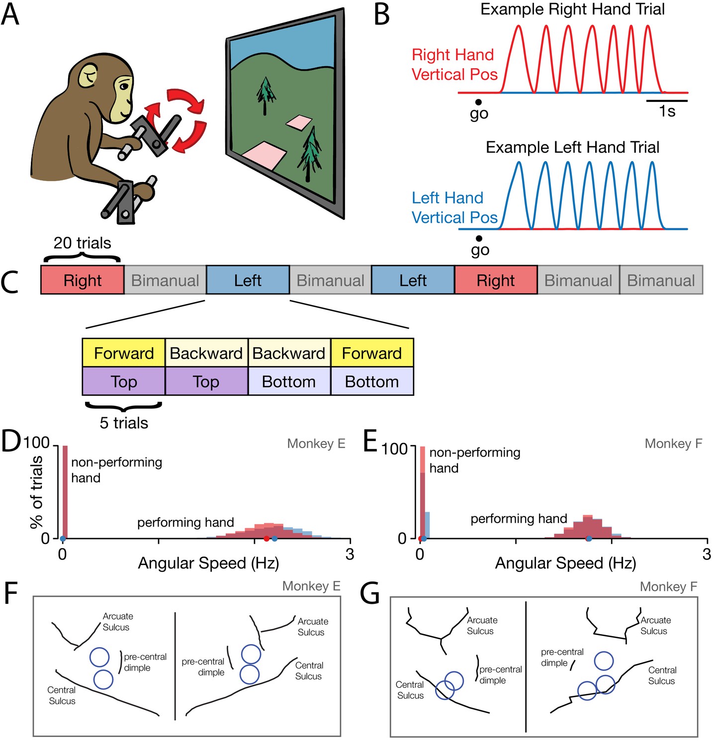
Behavior.
(A) Task schematic. Cycling one of the two pedals produced progress through a virtual environment. The other pedal had to remain stationary. This schematic simplifies the physical setup. In particular, pedals employed a handle that ensured consistent hand posture and a brace that minimized wrist movement. (B) Behavior on two example trials. After a go cue, the monkey cycled for seven cycles with one hand while holding the other hand stationary. Red trace: Right hand vertical position. Blue trace: Left hand vertical position. (C) Task structure. Blocks of right hand, left hand, and bimanual conditions were presented in pseudorandom order. Within each block of 20 trials, trials were presented in sub-blocks of five trials. There was one sub-block for each combination of cycling direction and starting position. (D) Distributions of cycling speed for the performing and non-performing hands. Distributions are across trials. Within each trial, the average angular speed was computed after taking the magnitude of velocity at each time. Red: Right hand. Blue: Left hand. Dots show distribution medians. Data are for Monkey E. (E) Same as D but for Monkey F. (F) For Monkey E, location of burr holes from which recordings were made, superimposed on MR-derived anatomical map. (G) Same as F, for Monkey F.
Figure 2

Two-step trial alignment procedure.
(A) Vertical hand position on all trials (within one session) for an example condition. Data are aligned to the first half-cycle of movement. Trials are colored green to purple based on the average cycling speed for that trial. (B) Raster plot of spike times for an example neuron, for the same trials shown in A. Trials are ordered by average cycling speed and aligned as in A. (C) Hand position traces after the second alignment step: adjusting the time-base of each trial so that cycling during the middle six cycles matched the typical 2 hz pedaling speed. (D) Spike times after the second alignment step. (E) Average firing rate calculated after the second alignment step. Black: Mean firing rate. Gray shading: standard error across trials. Label at bottom right gives neuron identity.
Figure 3
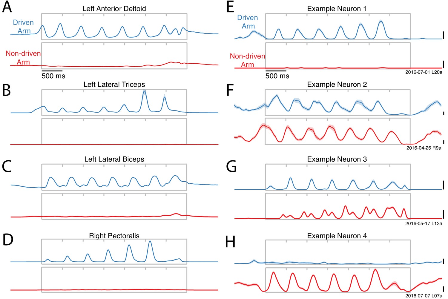
Activity versus time for four example muscles (A–D) and four example neurons (E–H).
Each panel shows activity for one condition performed with either the driven arm (blue) or the non-driven arm (red). Each trace plots trial-averaged activity, with flanking envelopes (sometimes barely visible) showing standard errors. Gray boxes indicate when the pedal was moving, with tick marks dividing each cycle. All examples are from Monkey E. Example neural recordings were from single-unit isolations for all figures (population analyses include single- and multi-unit isolations). Calibration bars are 10 spikes/s. For the muscles, the vertical scale is arbitrary but conserved within each panel.
Figure 4
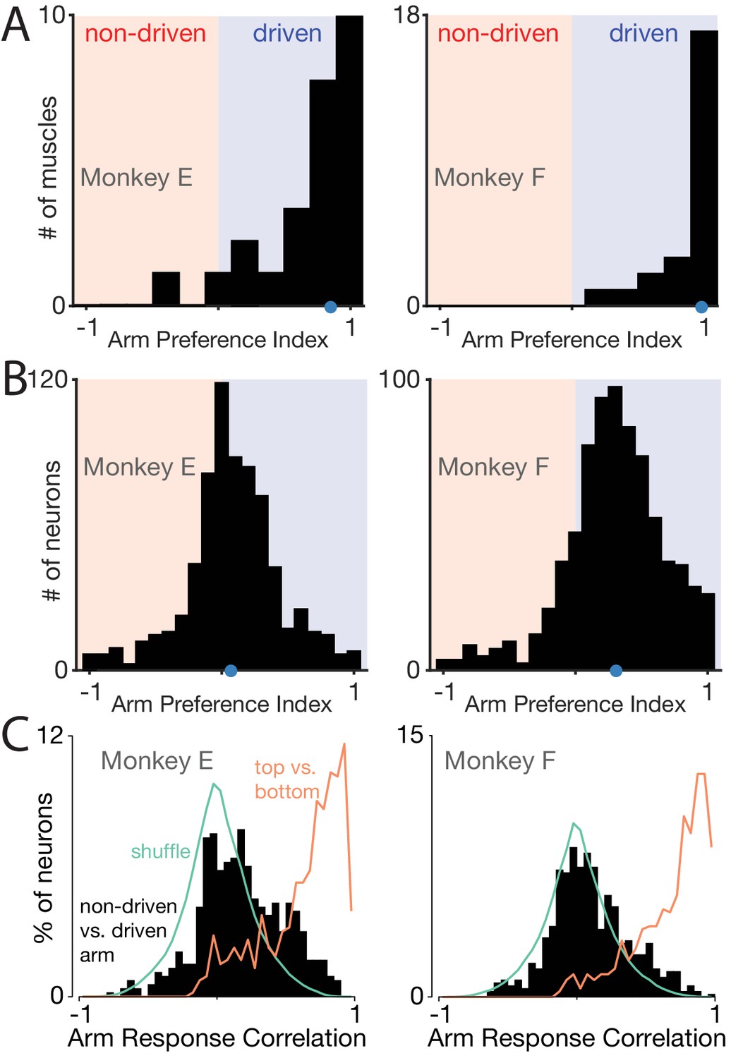
Muscle responses are lateralized while neural responses are not.
(A) Histograms of arm preference index for all recorded muscles. Shaded regions indicate preference for the non-driven arm (red) and driven arm (blue). Blue dot indicates the median. (B) Histograms of arm preference index for all recorded neurons. (C) Histograms summarizing, for single neurons, similarity of responses when the task is performed with the driven versus non-driven arm. For each neuron, we computed the correlation between those two responses. Black histograms plot the distribution of such correlations across all neurons. Orange trace: control demonstrating that high correlations are observed, as expected, when comparing responses during top-start versus bottom-start conditions. Green trace: distribution of correlations between pairs of different units. This distribution illustrates the range of incidental correlations observed if there is no tendency for responses to be similar, other than being drawn from the same overall set of responses.
Figure 5
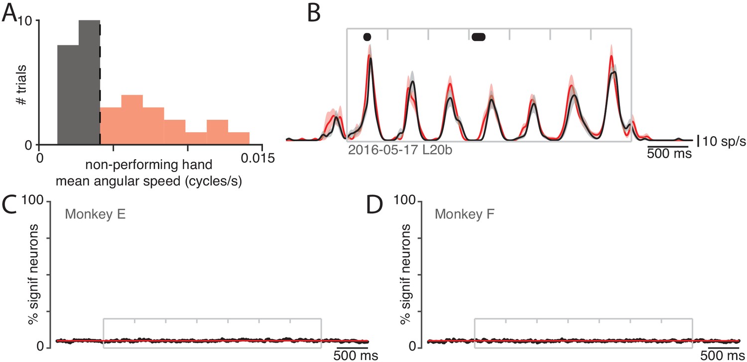
Small movements of the non-performing arm cannot explain modulation of neural activity within the non-driving cortex.
(A) Analysis employed the distribution (across trials) of the mean angular speed of the non-performing arm. This distribution is shown for one condition, recorded on 1 day. Trials were divided into those with mean speed less than (gray) or greater than (red) the median (vertical dashed line). (B) Firing rate of one example neuron for these two groups: trials with speeds less than (black) and greater than (red) the median. Envelopes show standard errors of the mean. Black dots at top indicate times when the two rates were significantly different (). Plotting conventions as in Figure 3. (C) Percentage of neurons (black trace) showing a statistically significant difference () in firing rate between trials with speeds less than versus greater than the median. Differences occurred as often as expected by chance (red line at 5%). Gray box denotes the time of movement. Each tick mark delineates a cycle. Data are for monkey E. Analysis is based on 426 units. (D) As in C but for Monkey F. Analysis is based on 479 units.
Figure 6

Correlations between neurons depend on which arm is used.
(A) Average firing rates of two neurons (green and orange traces) during one condition, performed with the driven arm (top pair of traces) and non-driven arm (bottom pair of traces). Responses are shown for the middle cycles, which form the basis of the analysis below. For this example, the firing rates of the two neurons were strongly correlated when the driven arm performed the task, and remained so when the non-driven arm performed the task. Shading shows standard errors of the mean. (B–D) Responses of three other pairs of neurons. All pairs exhibit correlated responses when the task was performed with the driven arm. Correlations disappear or even invert when the task is performed with the non-driven arm. (E) Pairwise correlations between all units recorded from the left hemisphere of monkey E. Each panel plots the correlation matrix for one condition, indicated at top. Ordering of units was based on data in the left panel, and is preserved across panels. (F) same but for Monkey F. (G) Scatterplots of pairwise correlations. Each dot corresponds to a pair of units for a given condition, and plots the firing rate correlation when using the non-driven arm versus that when using the driven arm. To aid visualization, a randomly-selected 1% of data points are shown. (H) Density plot of pairwise correlations for Monkey E (left) and Monkey F (right).
Figure 7 with 1 supplement
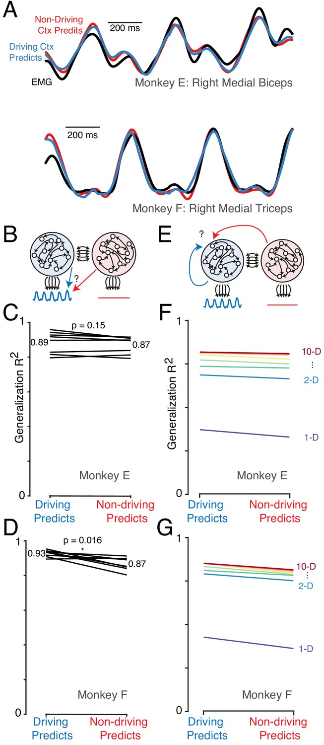
The dominant signals are very similar in the driving and non-driving cortex.
(A) Example muscle activity patterns (black) and predictions of muscle activity based on a linear decode of neural activity in the driving (blue) and non-driving (red) cortex. Examples are shown for one muscle from each monkey. In both cases, data is from a test condition and illustrates generalization performance. (B) Cartoon illustrating the analysis approach for comparing muscle-decode performance from the driving versus non-driving cortex. Performing-arm muscle activity (blue trace) is a product of descending connections (black arrows) from neurons within the driving cortex (blue network). It should thus be possible to predict (blue arrow) that muscle activity from neural activity recorded from the driving cortex. The presence or absence of muscle-like signals within the non-driving cortex (red network) was assessed by asking how well such activity predicted (red arrow) performing-arm muscle activity. (C) Prediction performance for the comparison illustrated in B. Data are for Monkey E. Each line corresponds to one behavioral condition and shows the percent variance (of muscle population activity) predicted by decodes based on driving and non-driving cortex neural activity. (D) As in C, for Monkey F. (E) Cartoon illustration of analysis asking whether the signals carried by the driving cortex are also present in the non-driving cortex. When the task is performed with a given arm, neural activity within the corresponding driving cortex is predicted either from the activity of other neurons either within the driving cortex (blue arrow) or within the non-driving cortex (red arrow). (F) Prediction performance for the comparison illustrated in E. Data are for Monkey E. Each color trace shows the average generalization performance across eight behavioral conditions for a given projection rank, using rainbow colors from red (10 dimensions) to purple (one dimension). Each line compares performance when predicting driving cortex activity from driving cortex activity (left) versus from non-driving (right). (G) As in panel F, for data from Monkey F.
Figure 7—figure supplement 1

Confirmation that the analysis in Figure 7C,D is sensitive to signal mismatch between driving and non-driving cortices, if that situation were present.
(A) Repetition of the analysis from the manuscript after altering activity within the non-driving cortex by removing the signal captured by the top PC. We did so by reconstructing each neuron’s response from all PCs (which would normally provide a perfect reconstruction) except the first. We took the original data matrix (with one column per neuron) and replaced it with , where is the matrix of PCs with the first column missing. Following this manipulation, generalization was lower when predicting the activity of driving-cortex neurons from non-driving-cortex neurons, rather than driving-cortex neurons (lines slope downwards). This pronounced decline is in contrast to the very modest decline observed in the data (see Figure 7F,G). (B) As in A, but using a different manipulation of non-driving cortex activity. Instead of removing signals, we created a mismatch in the size of signals in the driving versus non-driving cortex by manipulating the latter. We projected the original data matrix into its PC space, yielding . We divided the first two columns of by two, and multiplied columns three and four by two, yielding . We then reconstructed the activity of each neuron: and analyzed . Thus, all signals are present in both hemispheres, but to different degrees. Again, this creates a mismatch in generalization when predictions are based on driving- versus non-driving-cortex activity. These results illustrate that the original analysis can reveal if a signal is present in the driving-cortex, but absent, or of a different magnitude, in the non-driving cortex. Thus, the results of the original analysis indicate that any such differences are modest and/or restricted to higher PCs that capture relatively little variance.
Figure 8
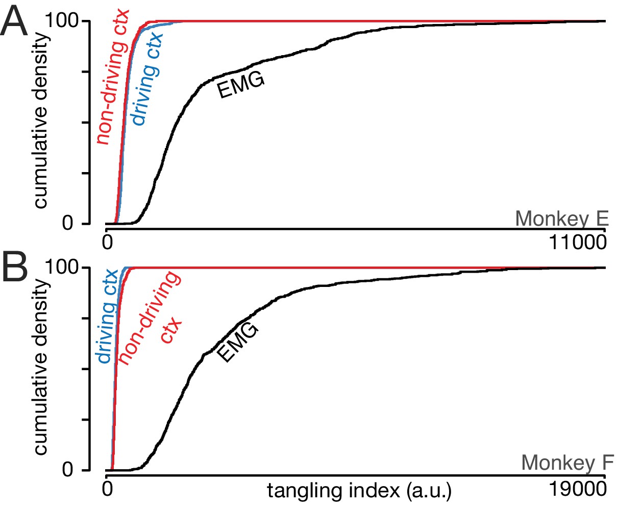
Trajectory tangling is similar for the driving and non-driving cortices.
(A) Cumulative distribution of trajectory tangling for the driving cortex (blue), non-driving cortex (red), and muscle activity (black). Distributions were compiled across time points and conditions. Data for Monkey E. (B) As in A, for Monkey F.
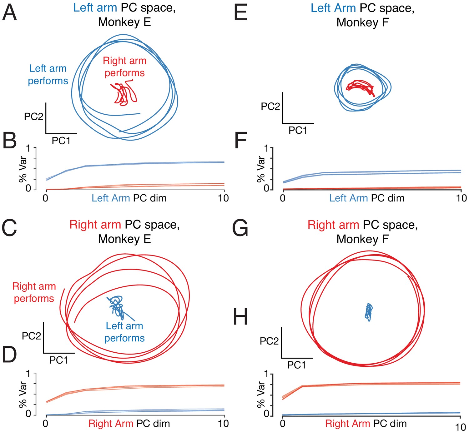
Figure 9 with 2 supplements
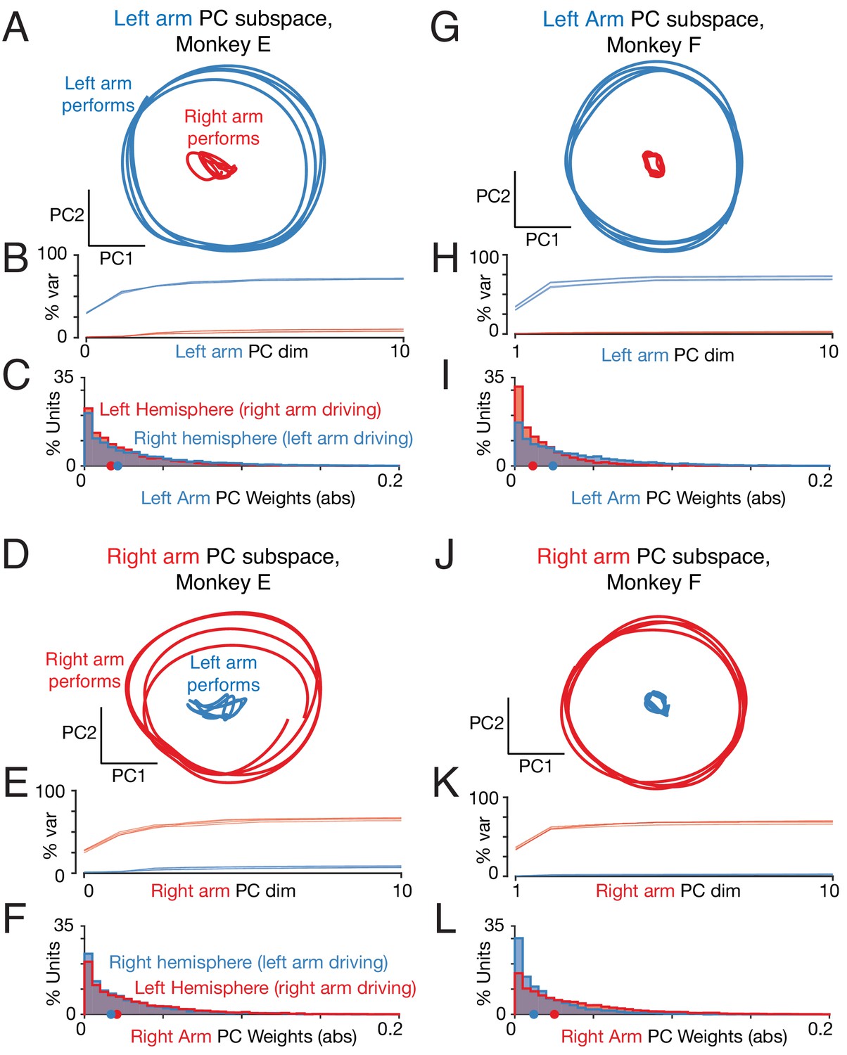
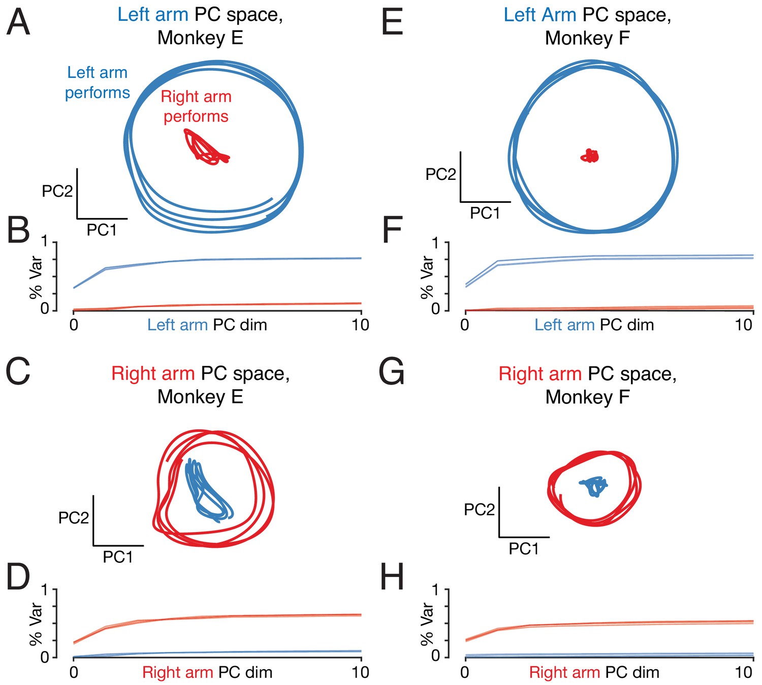
Left-arm and right-arm related activity lie in orthogonal subspaces.
(A) Projection of population activity onto the first two dimensions of the left-arm subspace. The left-arm subspace was found based on data from one condition (forward, top-start) performed with the left arm. This same subspace captured responses during another condition (forward, bottom-start) performed by the left arm (blue trajectory), but not for a condition (forward, top-start) performed with the right arm (red trajectory). Analysis considers data from the middle cycles, and all recorded neurons from both hemispheres. Data are for monkey E. (B) Cumulative percent variance explained by the left-arm subspace, for responses recorded when the left (blue) or right (red) arms performed the task. Variance explained was always computed for the left-out conditions (conditions not used to find the space). The analysis was performed with each condition serving as the training condition (used to find the space) once. There were four such conditions (two directions by two starting positions), yielding four (largely overlapping) traces of each color. Data are for monkey E. (C) Magnitude of the contribution to the left-arm subspace from units in the right (driving) and left (non-driving) hemispheres. A rightwards shift would indicate greater contribution from that hemisphere. Distribution medians are indicated by red and blue dots. The distribution was based on the absolute value of the weights contained in the top five PCs (after which the percent variance captured had largely plateaued). Histograms are combined across all behavioral conditions, so each neuron contributes 4 conditions x 5 PCs = 20 weights. (D–F) As in A-C, for the ‘right arm’ subspace. Note that the data projected are the same as in panel A – only the subspace differs. (G–L) As in A-F, for Monkey F.
Figure 9—figure supplement 1
Repetition of analysis in Figure 9, but analyzing the neural population from the right cortex only.
Right-cortex activity is modestly stronger when performing the task with the left versus right arm. Trajectories when the left arm performs the task (blue traces) are thus magnified modestly relative to trajectories when the right arm performs the task (red traces). This increases the magnitude difference between left-arm performing and right-arm performing trajectories in the left-arm space (top; a modest increase in the effect compared to analysis of the full population) and modestly reduces the magnitude in the right-arm space (top; a modest decrease in the effect compared to analysis of the full population). This effect actually aids the (presumed) goal of ignoring ‘wrong-arm’ related activity. The neural population being analyzed is recorded from the right hemisphere (and thus drives the left arm). Ignoring wrong-arm activity thus requires that there be little occupation of the left-arm space when the right arm performs the task. This is indeed the scenario in which there is the largest difference in occupancy between the two arms (the effect is larger in panels A and E versus C and G). Thus, two effects – orthogonality of subspace and modestly greater activity when using the contralateral arm – both potentially aid the ability to control the arms independently.
Figure 9—figure supplement 2
Repetition of analysis in Figure 9, but analyzing the neural population from the left cortex only.
Same as Figure 9—figure supplement 1 in all other respects.
Figure 10 with 1 supplement
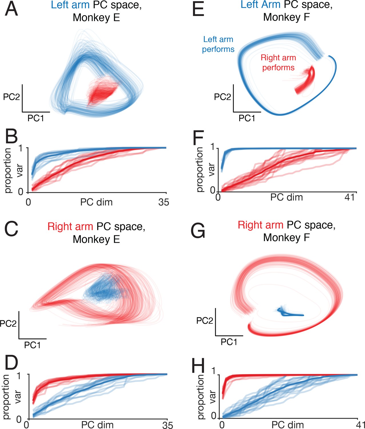
Left-arm and right-arm related activity on single trials.
(A) Similar analysis to that in Figure 9A, but projecting single-trial firing rates inferred using LFADS. Each trace plots the projection of the population response during one cycle of one trial (both top-start and bottom-start conditions are shown). Data are for one session performed by monkey E. (B) Cumulative proportion of variance explained by the left-arm subspace, for single-trial responses recorded when the left (blue) or right (red) arms performed the task. Each recording session contributes four traces: one for each pedaling direction and performing arm. The dark trace shows the average. The proportion of variance was normalized to always be unity for 35 PCs (corresponding to the maximum population size across all included datasets for this monkey), to allow comparison across sessions with different numbers of isolations. (C) The same example trials shown in A, projected onto the first two dimensions of the right-arm subspace. (D) As in B, for cumulative percentage variance explained by the right-arm subspace. (E–H) As in A-D, for Monkey F.
Figure 10—figure supplement 1

High cell-counts help to reliably reveal when neural subspaces are orthogonal.
We used the ‘alignment index’ (see below) to assess orthogonality of subspaces. Perfectly aligned subspaces have an alignment index of unity, and perfectly orthogonal subspaces have an alignment index of zero. We used the alignment index to compare subspaces where the right versus left arm performed the task (purple) and where cycling started at the top versus the bottom (green). The alignment index was computed for populations of different sizes, found by subsampling the original population. Lines and shading show means ± standard deviations across 100 random subsamples per condition. Panels A and B show the analysis for monkeys E and F. The orthogonality of right- versus left-arm subspaces became increasingly clear with higher neuron-counts. This (along with increased sampling noise) is likely one reason why orthogonality was slightly weaker for single-trial analyses. In contrast, top-start and bottom-start subspaces were well-aligned regardless of population size. The alignment index was defined as: , where is the matrix of firing rates of all neurons during a given condition. is the vector of projection weights for Principal Component , for PCA run on X. is the projection weight vector for dimension of PCA run on the comparison condition (either other arm or other start position). PCA and alignment indices were computed for each behavior (start position, cycling direction) individually. For example when computing the alignment index between right- and left-arm subspaces, this was done separately for each combination for forward/backward and top-start/bottom-start. Results were then averaged across conditions (and random subsamples, as described above).
Figure 11 with 2 supplements
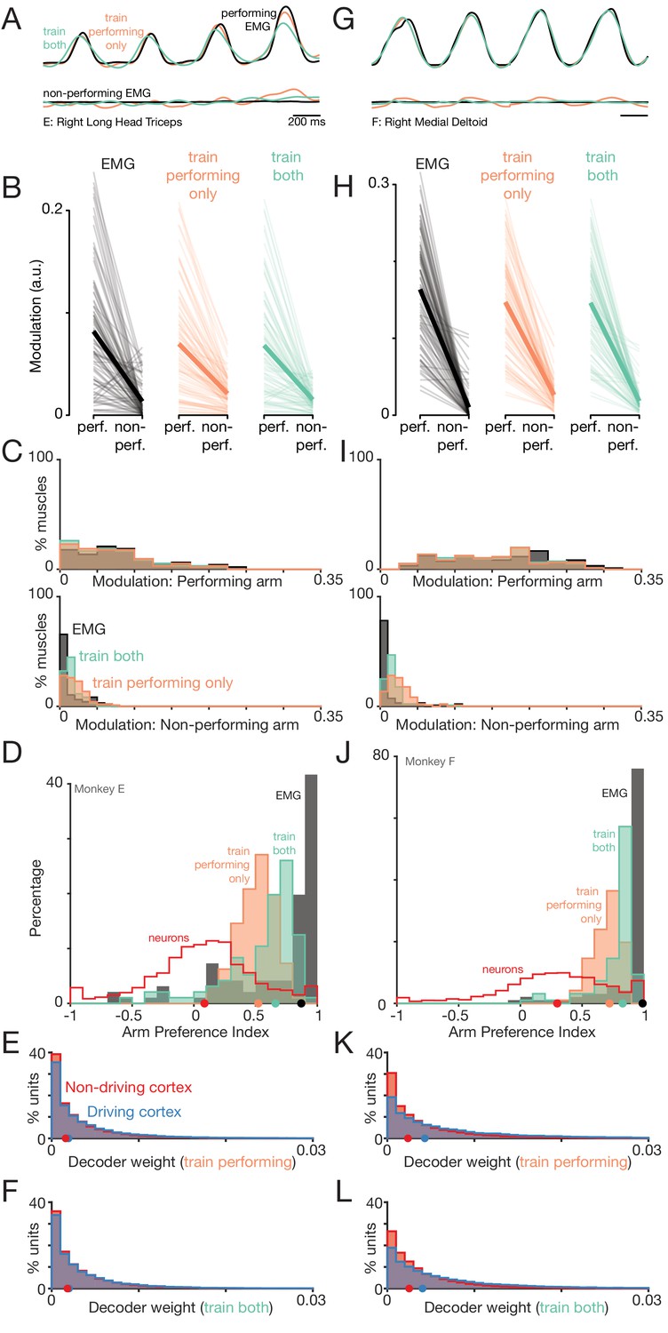
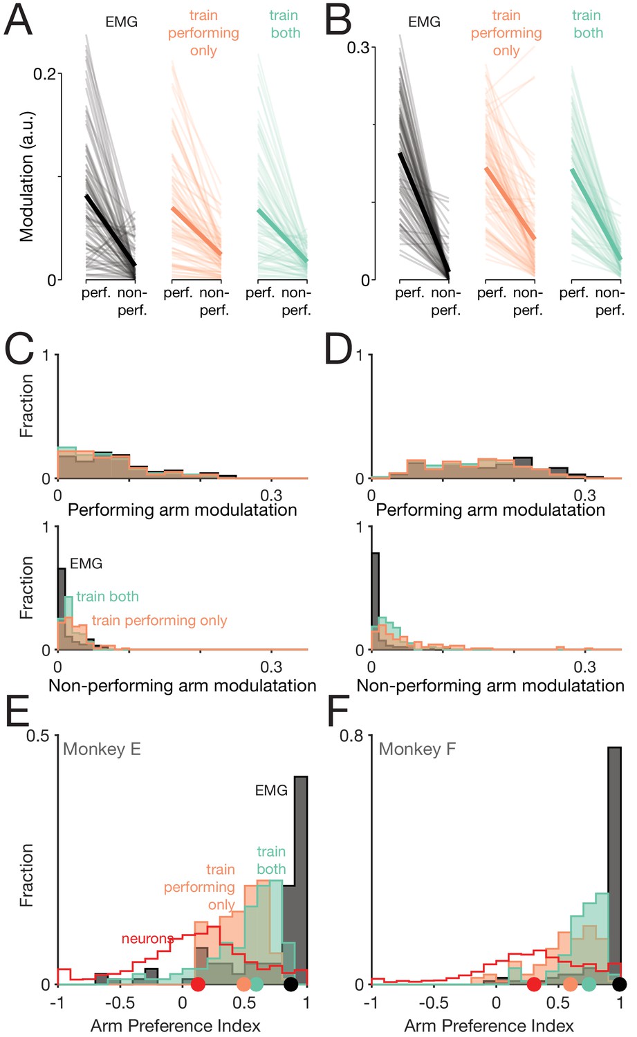
Muscle-activity decoders ignore activity related to the ‘wrong’ arm.
(A) Actual (black) and predicted activity of the long head of the triceps, recorded from the right arm of monkey E. Top traces: activity while the right arm performed the task. Bottom traces: activity while the left arm performed the task. Orange traces: Predictions of a decoder trained only on right-arm-performing conditions (‘train-performing-only’ decoder). Green traces: Predictions of a decoder trained on a subset of both left- and right-arm-performing conditions (‘train-both’ decoder). Both the top and bottom responses are from a held-out condition on which decoders were not trained. (B) Actual and predicted modulation of muscle activity when the task is performed using the arm containing that muscle (perf.) or with the other arm (non-perf.). Each thin line plots the modulation for one muscle during one condition (e.g. the deltoid, for top-start forward cycling). Thick lines show medians. The three subpanels correspond to the empirical muscle activity, the train-performing-only decoder (trained only conditions where the task was performed by the arm containing the muscle), and the train-both decoder (trained on conditions of both types). Modulation was always measured for predictions of muscle activity during held-out conditions, for which decoders had to generalize. Data are for monkey E. (C) Same data as in B, but plotted in distribution form. Each histogram plots the distribution of empirical (black) or predicted (orange and green) muscle activity across all muscles/conditions. Distributions are plotted separately when the decoded muscle was in the performing (top) or non-performing arm (bottom), to aid comparison within each situation. (D) Distribution of arm preference indices for neurons (red), muscles (gray), predictions of a decoder trained only on performing-arm conditions (orange), and predictions of a decoder trained on both performing and non-performing arm conditions (green). Data are for monkey E. Red and gray histograms differ slightly from those in Figure 4A–B as they are computed per condition, given that the present analysis focuses on generalization performance for left-out conditions. (E) Distribution of decoder weight magnitudes (the contribution of each neuron to decode of muscle activity) for driving-cortex (blue) and non-driving-cortex (red) neurons. Weights are for train-performing-only decoders. Dots show distribution medians. (F) As in E, for train-both decoders. (G–L) As in A-F, for Monkey F.
Figure 11—figure supplement 1
Repetition of analysis in Figure 11, analyzing the neural population from the right hemisphere only.
https://doi.org/10.7554/eLife.46159.017
Figure 11—figure supplement 2

Repetition of analysis in Figure 11, analyzing the neural population from the left hemisphere only.
https://doi.org/10.7554/eLife.46159.018
Author response image 1

Figure 4 variant: Neural responses are not strongly lateralized (restricted to neurons from posterior burr holes).
(A) Histograms of arm preference index for all recorded neurons from posterior burr holes. (C) Histograms summarizing, for single neurons, similarity of responses when the task is performed with the driven versus non-driven arm. For each neuron, we computed the correlation between those two responses. Black histograms plot the distribution of such correlations across all neurons. Orange trace: control demonstrating that high correlations are observed, as expected, when comparing responses during top-start versus bottom-start conditions. Green trace: expected distribution if there is no special relationship between responses corresponding to the two arms. This was computed as the correlation between each non-matched pair of neurons.
Author response image 2
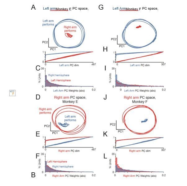
Figure 9 variant: Left arm and right arm related activity lie in orthogonal subspaces.
(A) Projection of population activity during an example condition performed by the left arm (blue) and the same behavior performed by the right arm (red), with PCs found using only data during left arm movement. The neural population includes all recorded neurons from both hemispheres, restricted to the posterior burr holes. Analysis considers data from the middle cycles. PCs were found using one behavioral condition, and data shown is from held-out conditions projected into the PC space: either for the condition with the same pedaling direction and hand, but opposite start position, or for the condition with the same start position and pedaling direction, but other hand. Data are for monkey E. (B) Cumulative percent variance explained during conditions performed by the left arm (blue) and conditions performed by the right arm (red), with PCs found using only data during left arm movement. The neural population includes all recorded neurons from both hemispheres, restricted to posterior burr holes. PCs were found using one behavioral condition, and variance explained is assessed on held-out conditions: either the same pedaling direction and performing arm, but opposite start position, or for the same start position and pedaling direction, but opposite performing arm. Each trace is a different generalization condition (four total per arm). Data are for Monkey E. (C) Distribution of the absolute value of neuron weights onto the first five “left arm” PCs. Blue traces: units in the right hemisphere (that drive the left arm). Red: units in the left hemisphere (driving the right arm). Histograms are combined across all behavioral conditions, so each neuron contributes 4 conditions x 5 PCs = 20 weights. (G-L) As in A-F, for Monkey F.
Additional files
-
Transparent reporting form
- https://doi.org/10.7554/eLife.46159.019
Download links
A two-part list of links to download the article, or parts of the article, in various formats.
Downloads (link to download the article as PDF)
Open citations (links to open the citations from this article in various online reference manager services)
Cite this article (links to download the citations from this article in formats compatible with various reference manager tools)
Motor cortex signals for each arm are mixed across hemispheres and neurons yet partitioned within the population response
eLife 8:e46159.
https://doi.org/10.7554/eLife.46159


