A consensus guide to capturing the ability to inhibit actions and impulsive behaviors in the stop-signal task
- Ghent University, Belgium
- University of California, San Diego, United States
- Leiden University, Netherlands
- Dresden University of Technology, Germany
- Stanford University, United States
- University of Maryland, United States
- Indiana University, United States
- University of Cambridge, United Kingdom
- Cardiff University, United Kingdom
- Oldenburg University, Germany
- University of Western Ontario, Canada
- Monash University, Australia
- University of Toronto, Canada
- University of Vermont, United States
- University of Oregon, United States
- University of Tasmania, Australia
- University of Oslo, Norway
- Spinoza Centre Amsterdam, Netherlands
- Utrecht University, Netherlands
- KU Leuven, Belgium
- Yale University, United States
- Vanderbilt University, United States
- University of Amsterdam, Netherlands
- Anglia Ruskin University, United Kingdom
- Indian Institute of Science, India
- Queen's University, Canada
- King's College London, United Kingdom
- Michigan State University, United States
- University of Iowa, United States
- Trinity College Dublin, Ireland
- Donders Institute, Netherlands
Figures
Figure 1
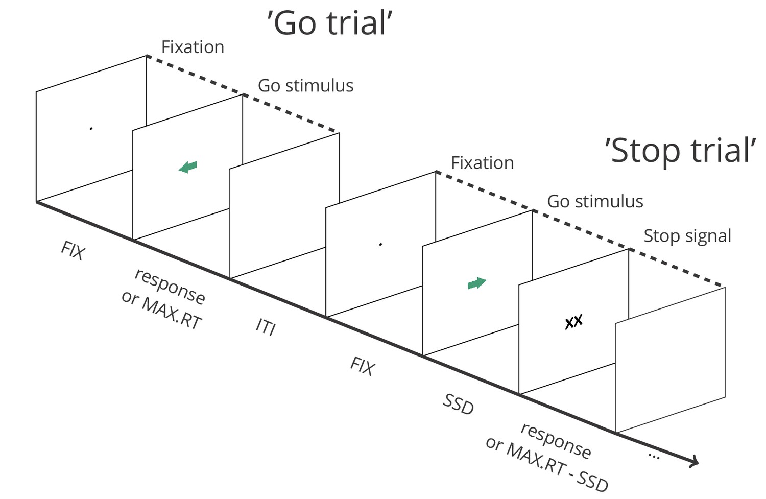
Depiction of the sequence of events in a stop-signal task (see https://osf.io/rmqaw/ for open-source software to execute the task).
In this example, participants respond to the direction of green arrows (by pressing the corresponding arrow key) in the go task. On one fourth of the trials, the arrow is replaced by ‘XX’ after a variable stop-signal delay (FIX = fixation duration; SSD = stop signal delay; MAX.RT = maximum reaction time; ITI = intertrial interval).
Box 1—figure 1
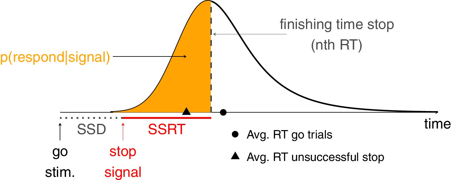
The independent race between go and stop.
https://doi.org/10.7554/eLife.46323.004
Figure 2
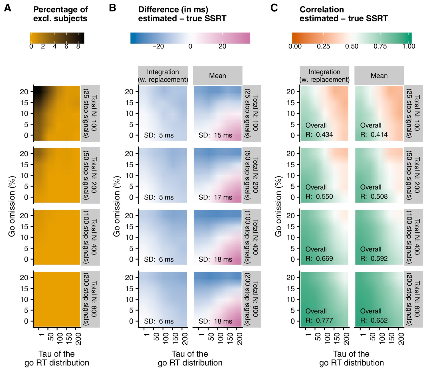
Main results of the simulations reported in Appendix 2.
Here, we show a comparison of the integration method (with replacement of go omissions) and the mean method, as a function of percentage of go omissions, skew of the RT distribution (), and number of trials. Appendix 2 provides a full overview of all methods. (A) The number of excluded ‘participants’ (RT on unsuccessful stop trials RT on go trials). As this check was performed before SSRTs were estimated (see Recommendation 7), the number was the same for both estimation methods. (B) The average difference between the estimated and true SSRT (positive values = overestimation; negative values = underestimation). SD = standard deviation of the difference scores (per panel). (C) Correlation between the estimated and true SSRT (higher values = more reliable estimate). Overall R = correlation when collapsed across percentage of go omissions and . Please note that the overall correlation does not necessarily correspond to the average of individual correlations.
Appendix 1—figure 1
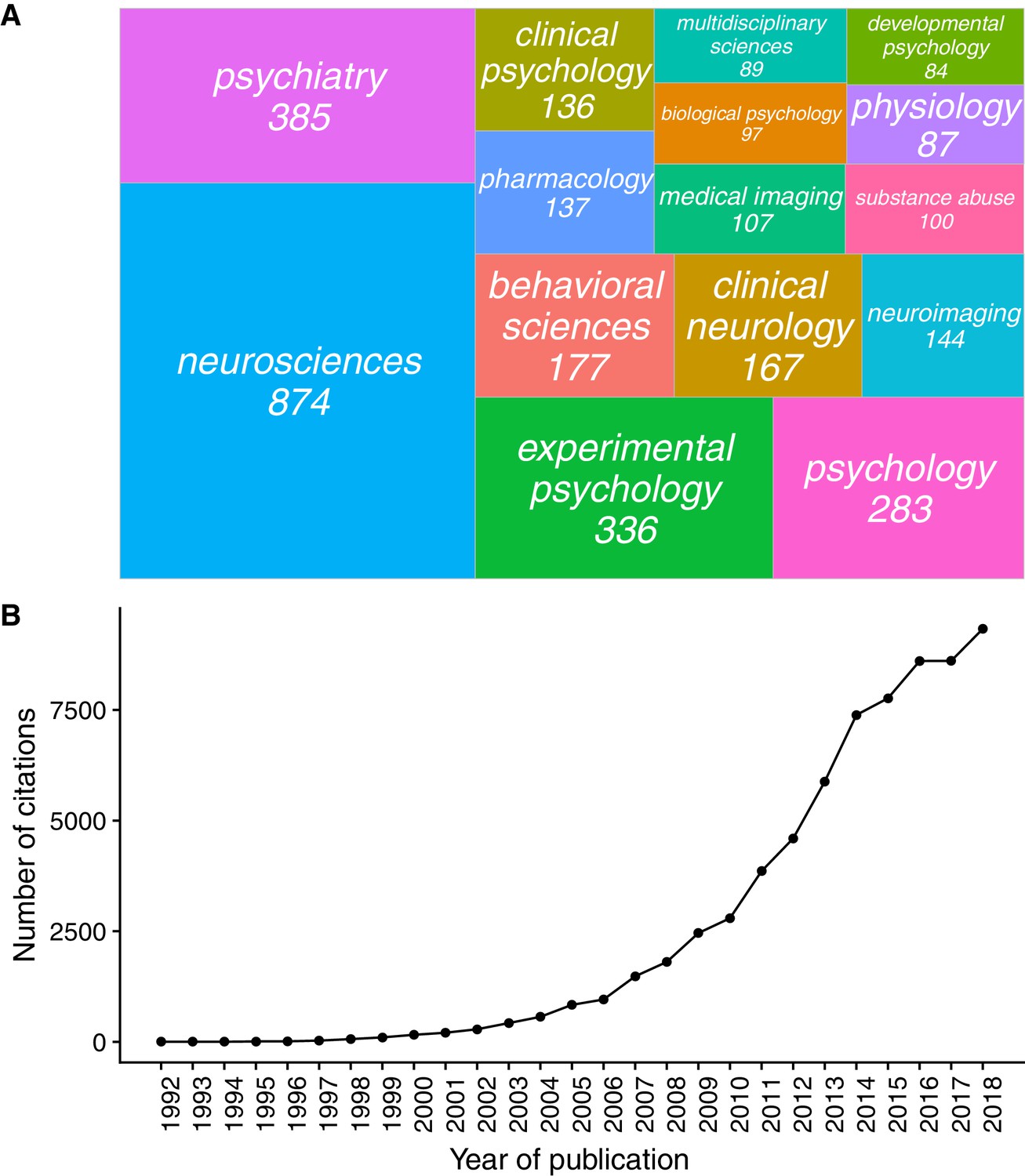
The number of stop-signal publications per research area (Panel A) and the number of articles citing the ‘stop-signal task’ per year (Panel B).
Source: Web of Science, 27/01/2019, search term: ‘topic = stop signal task’. The research areas in Panel A are also taken from Web of Science.
Appendix 2—figure 1
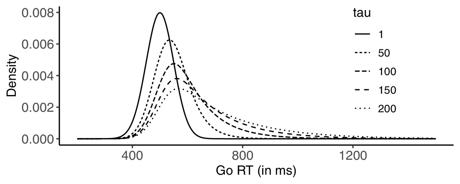
Examples of ex-Gaussian (RT) distributions used in our simulations.
For all distributions, = 500 ms, and = 50 ms. was either 1, 50, 100, 150, and 200 (resulting in increasingly skewed distributions). Note that for a given RT cut-off (1,500 ms in the simulations), cut-off-related omissions are rare, but systematically more likely as tau increases. In addition to such ‘natural’ go omissions, we introduced ‘artificial’ ones in the different go-omission conditions of the simulations (not depicted).
Appendix 2—figure 2

Violin plots showing the distribution and density of the difference scores between estimated and true SSRT as a function of condition and estimation method when the total number of trials is 100 (25 stop trials).
Values smaller than zero indicate underestimation; values larger than zero indicate overestimation.
Appendix 2—figure 3
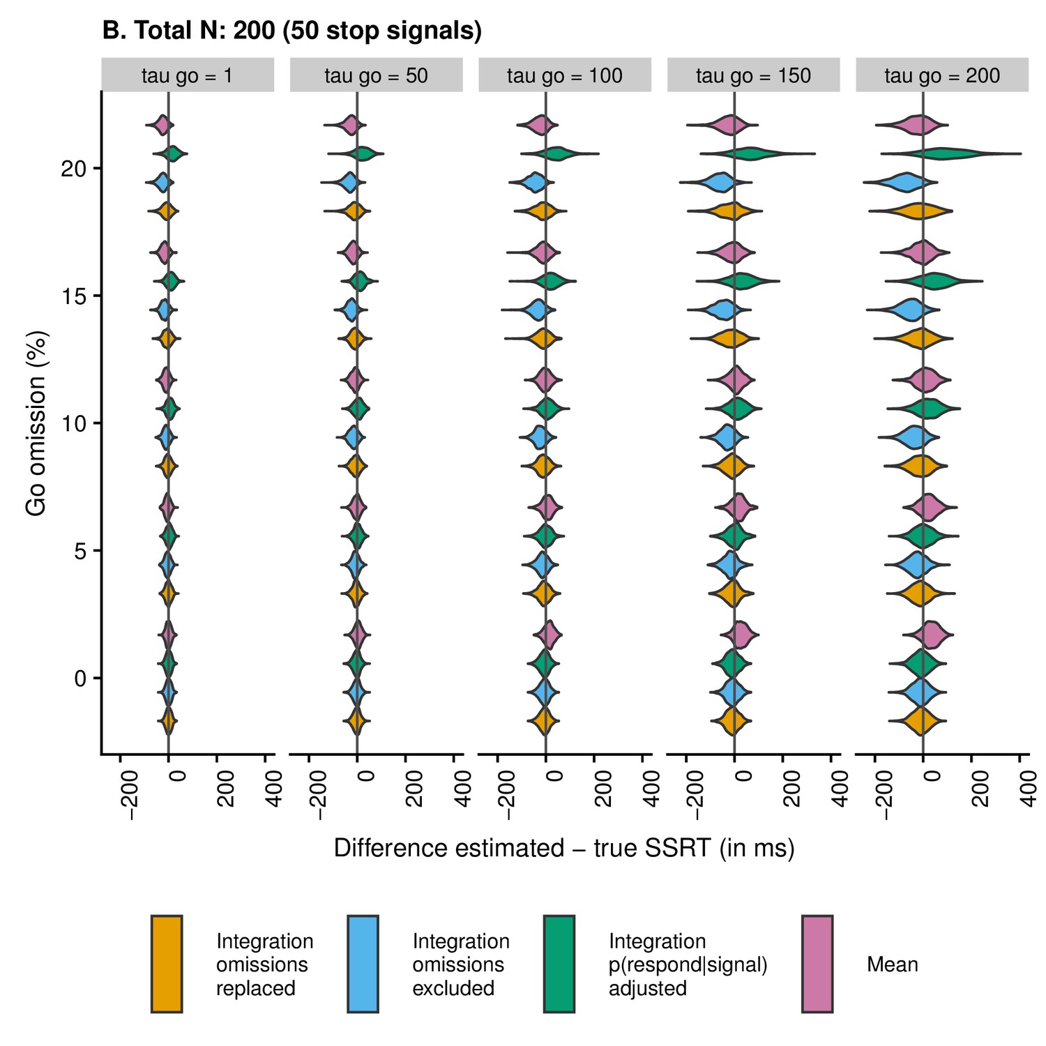
Violin plots showing the distribution and density of the difference scores between estimated and true SSRT as a function of condition and estimation method when the total number of trials is 200 (50 stop trials).
Values smaller than zero indicate underestimation; values larger than zero indicate overestimation.
Appendix 2—figure 4
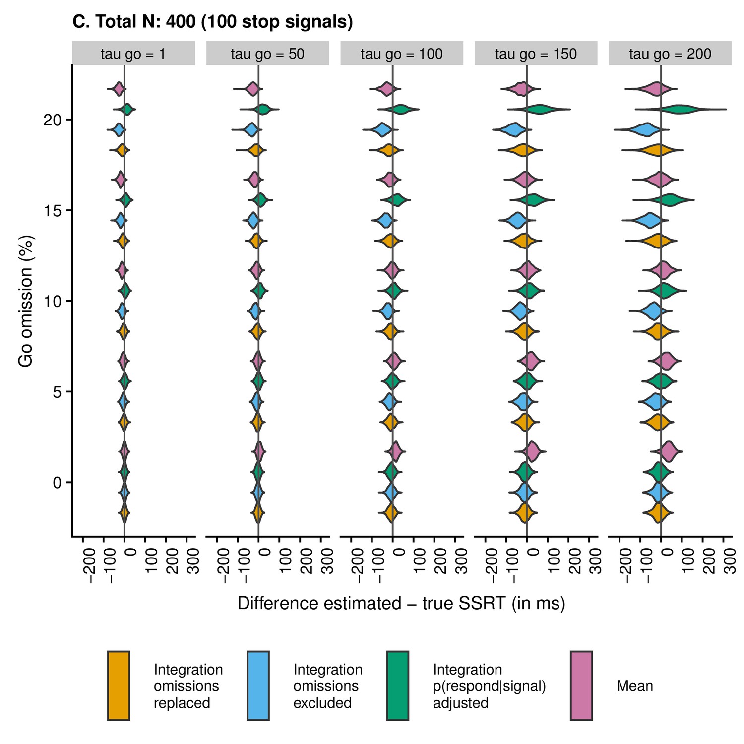
Violin plots showing the distribution and density of the difference scores between estimated and true SSRT as a function of condition and estimation method when the total number of trials is 400 (100 stop trials).
Values smaller than zero indicate underestimation; values larger than zero indicate overestimation.
Appendix 2—figure 5
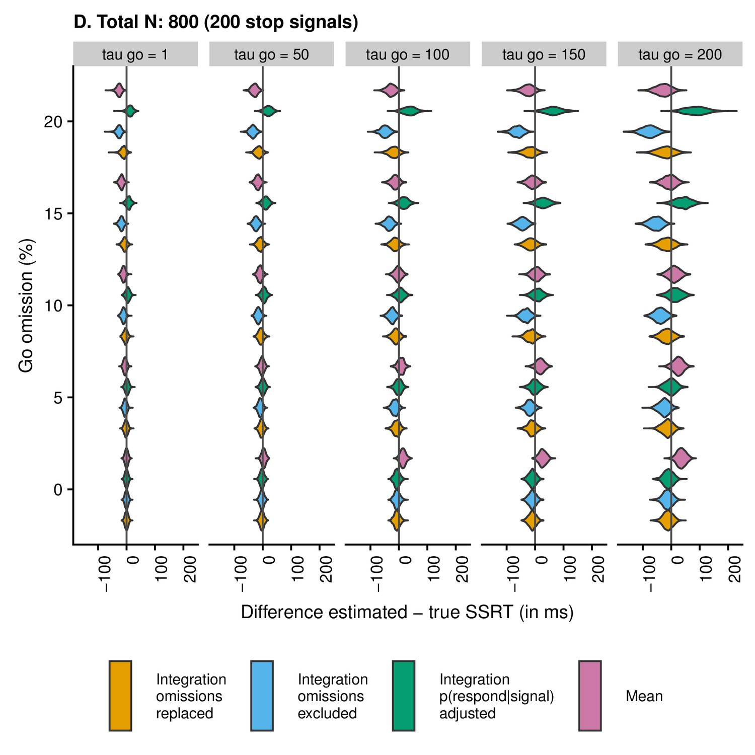
Violin plots showing the distribution and density of the difference scores between estimated and true SSRT as a function of condition and estimation method when the total number of trials is 800 (200 stop trials).
Values smaller than zero indicate underestimation; values larger than zero indicate overestimation.
Appendix 3—figure 1
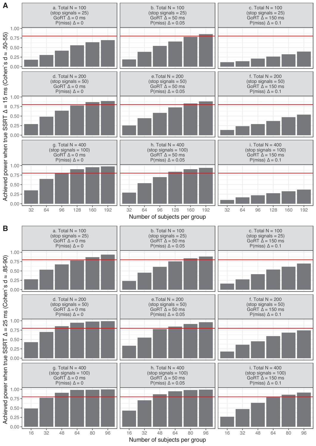
Achieved power for an independent two-groups design as function of differences in go omission, go distribution, SSRT distribution, and the number of trials in the ‘experiments’.
https://doi.org/10.7554/eLife.46323.020Tables
Appendix 2—table 1
The mean difference between estimated and true SSRT for participants who were included in the main analyses and participants who were excluded (because average RT on unsuccessful stop trials average RT on go trials).
We did this only for = 1 or 50, p(go omission)=10, 15, or 20, and number of trials = 100 (i.e. when the number of excluded participants was high; see Panel A, Figure 2 of the main manuscript).
| Estimation method | Included | Excluded |
|---|---|---|
| Integration with replacement of go omissions | −6.4 | −35.8 |
| Integration without replacement of go omissions | −19.4 | −48.5 |
| Integration with adjusted p(respond|signal) | 12.5 | −17.4 |
| Mean | −16.0 | −46.34 |
Appendix 3—table 1
Parameters of the go distribution for the control group and the three experimental conditions.
SSRT of all experimental groups differed from SSRT in the control group (see below).
| Parameters of go distribution | Control | Experimental 1 | Experimental 2 | Experimental 3 |
|---|---|---|---|---|
| 500 | 500 | 525 | 575 | |
| 50 | 50 | 52.5 | 57.5 | |
| 50 | 50 | 75 | 125 | |
| go omission | 0 | 0 | 5 | 10 |
Additional files
-
Transparent reporting form
- https://doi.org/10.7554/eLife.46323.007
Download links
A two-part list of links to download the article, or parts of the article, in various formats.
Downloads (link to download the article as PDF)
Open citations (links to open the citations from this article in various online reference manager services)
Cite this article (links to download the citations from this article in formats compatible with various reference manager tools)
A consensus guide to capturing the ability to inhibit actions and impulsive behaviors in the stop-signal task
eLife 8:e46323.
https://doi.org/10.7554/eLife.46323


