Choice history biases subsequent evidence accumulation
- University Medical Center Hamburg-Eppendorf, Germany
- University of Amsterdam, Netherlands
Figures
Figure 1

Two biasing mechanisms within the DDM.
The DDM postulates that noisy sensory evidence is accumulated over time, until the resulting decision variable y reaches one of two bounds (dashed black lines at y = 0 and y = a) for the two choice options. Repeating this process over many trials yields RT distributions for both choices (plotted above and below the bounds). Gray line: example trajectory of the decision variable from a single trial. Black lines: mean drift and resulting RT distributions under unbiased conditions. (a) Choice history-dependent shift in starting point. Green lines: mean drift and RT distributions under biased starting point. Gray-shaded area indicates those RTs for which starting point leads to choice bias. (b) Choice history-dependent shift in drift bias. Blue lines: mean drift and RT distributions under biased drift. Gray shaded area indicates those RTs for which drift bias leads to choice bias. (c) Both mechanisms differentially affect the shape of RT distributions. Conditional bias functions (White and Poldrack, 2014), showing the fraction of biased choices as a function of RT, demonstrate the differential effect of starting point and drift bias shift.
Figure 2

Behavioral tasks and individual differences.
(a) Schematics of perceptual decision-making tasks used in each dataset. See also Materials and methods section Datasets: behavioral tasks and participants. (b) Distributions of individual choice history biases for each dataset. Gray bars show individual observers, with colored markers indicating the group mean. (c) Each individual’s tendency to repeat their choices after correct vs. error trials. The position of each observer in this space reflects their choice- and outcome-dependent behavioral strategy.
Figure 3 with 2 supplements
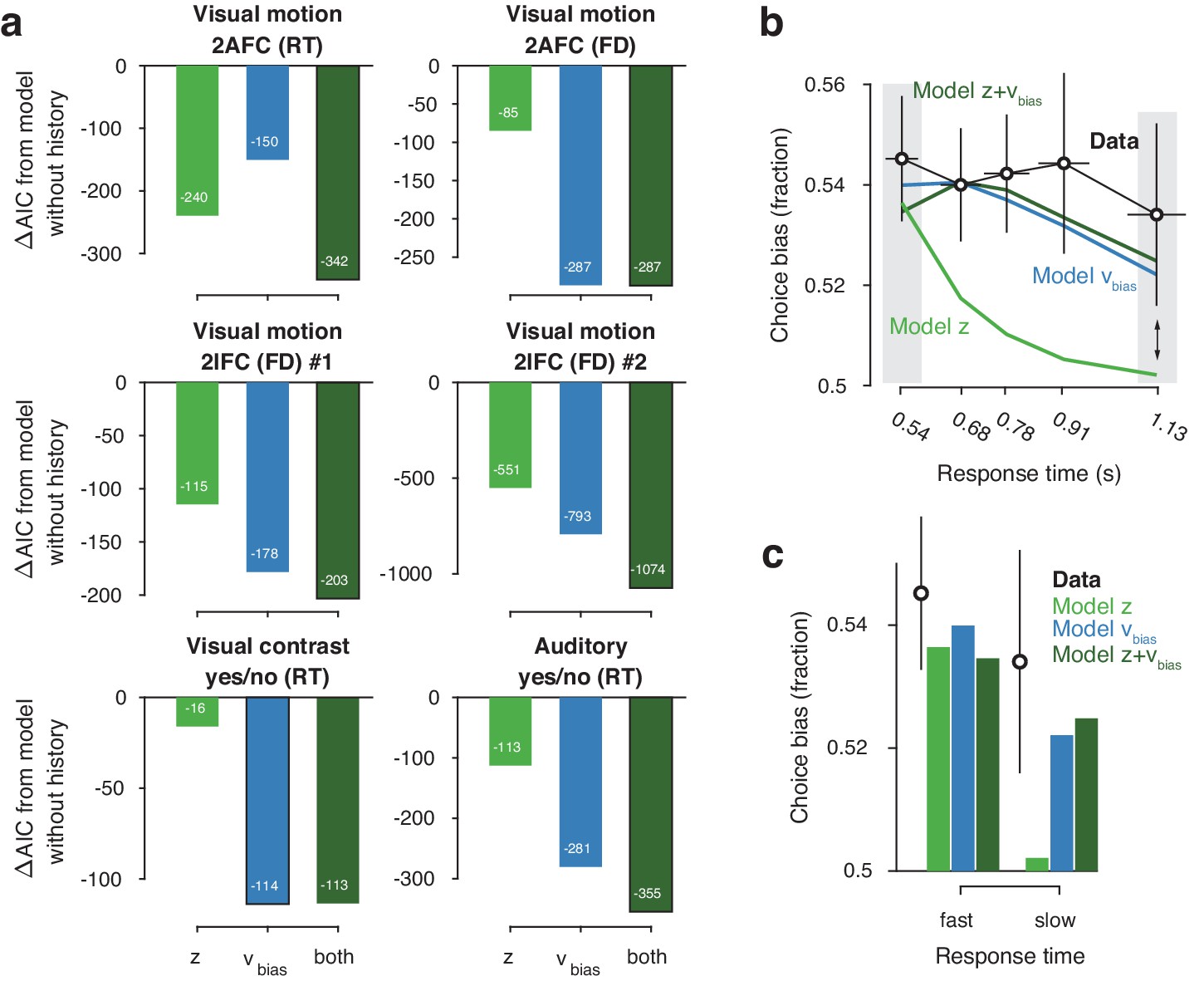
Model comparison and simulations.
(a) For each dataset, we compared the AIC between models where drift bias, starting point bias or both were allowed to vary as a function of previous choice. The AIC for a model without history dependence was used as a baseline for each dataset. Lower AIC values indicate a model that is better able to explain the data, taking into account the model complexity; a ΔAIC of 10 is generally taken as a threshold for considering one model a sufficiently better fit. (b) Conditional bias functions (Figure 1c; White and Poldrack, 2014). For the history-dependent starting point, drift bias and hybrid models, as well as the observed data, we divided all trials into five quantiles of the RT distribution. Within each quantile, the fraction of choices in the direction of an individual’s history bias (repetition or alternation) indicates the degree of choice history bias. Error bars indicate mean ± s.e.m. across datasets. (c) Choice bias on slow response trials can be captured only by models that include history-dependent drift bias. Black error bars indicate mean ± s.e.m. across datasets, bars indicate the predicted fraction of choices in the first and last RT quantiles.
Figure 3—figure supplement 1
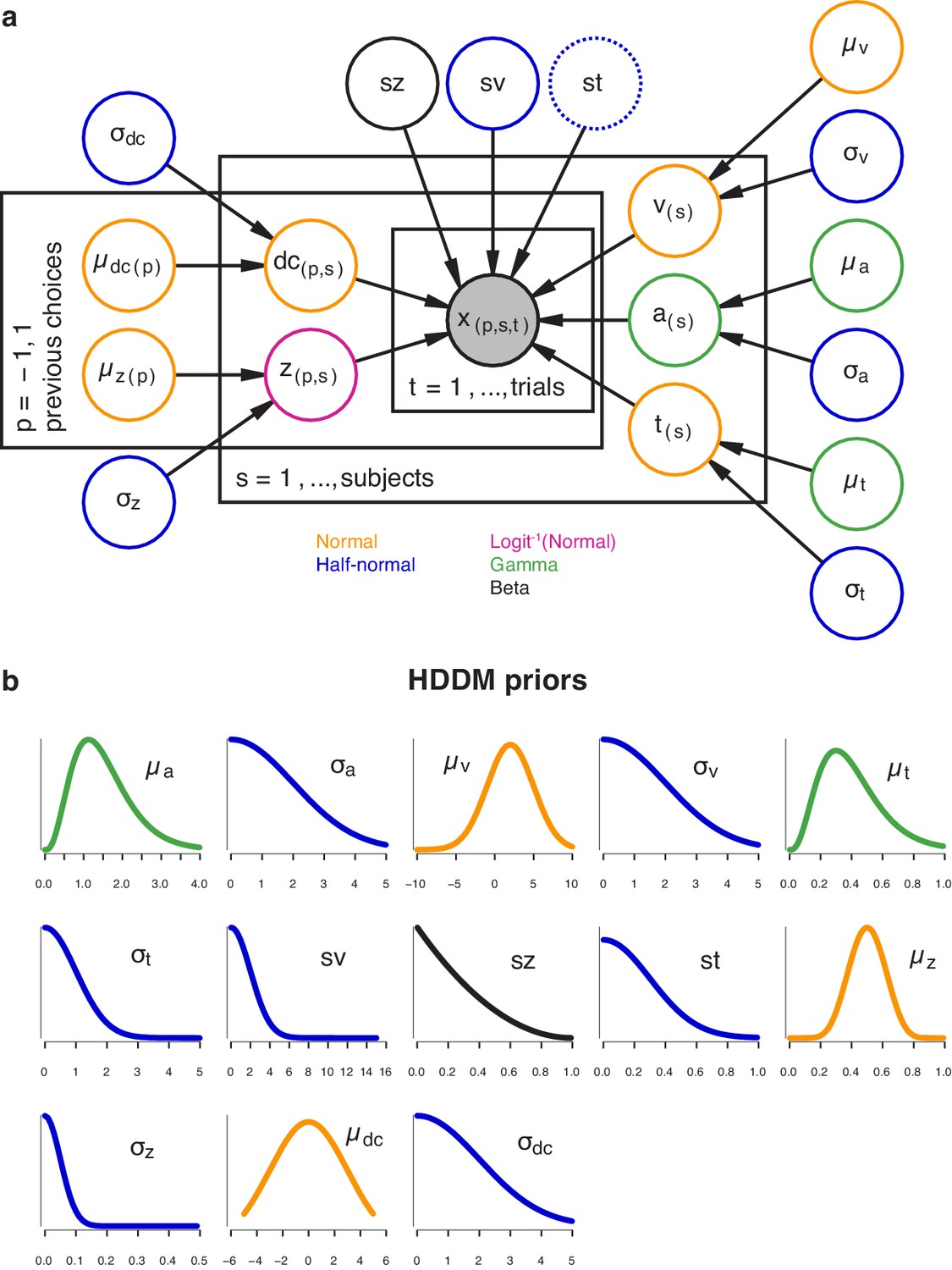
The hierarchical DDM.
(a) Graphical representation of the hierarchical model structure. The full model (with both history-dependent drift bias and starting point) is depicted. Round nodes represent random variables, and the shaded node x represented the observed data (choices and RTs for all observers within each task). Subject-specific parameter estimates were distributed according to the group-level posterior values, thereby ‘shrinking’ individual values toward the group average. Colors indicate the distributions used for each node. For the datasets with multiple stimulus difficulty levels, we additionally estimated a separate drift rate (v) for each (Figure 3—figure supplement 2a, inset). Between-trial variability in non-decision time was only included in the model shown in Figure 4—figure supplement 2b. (b) Prior distributions used for each node, with colors indicating their distribution. See (Wiecki et al., 2013) for the full set of prior specifications.
Figure 3—figure supplement 2
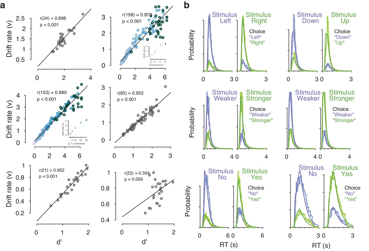
Drift diffusion model fits.
(a) Correlation between drift rate () and d’. In the two datasets with multiple stimulus difficulty levels (Visual motion 2AFC (FD) and Visual motion 2IFC (FD) #1), drift rates were estimated separately for each level of stimulus difficulty. In these two datasets, the correlation coefficient displayed is a partial correlation between and d’, while accounting for stimulus difficulty (inset, colors indicate discrete stimulus difficulty levels). As expected, the mean drift rate increased monotonically as a function of evidence strength. (b) Measured and predicted RT distributions, across all trials and observers within each dataset. Observed (light) and predicted (dark) RT distributions are separately shown for each combination of stimulus and choice (green/purple), with the low-probability distributions indicating error trials.
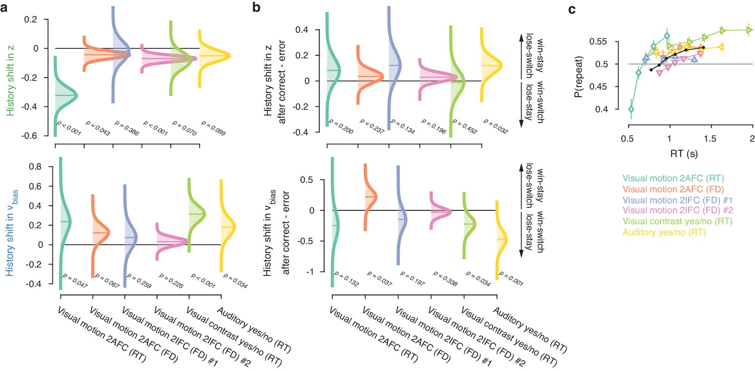
Figure 4 with 5 supplements
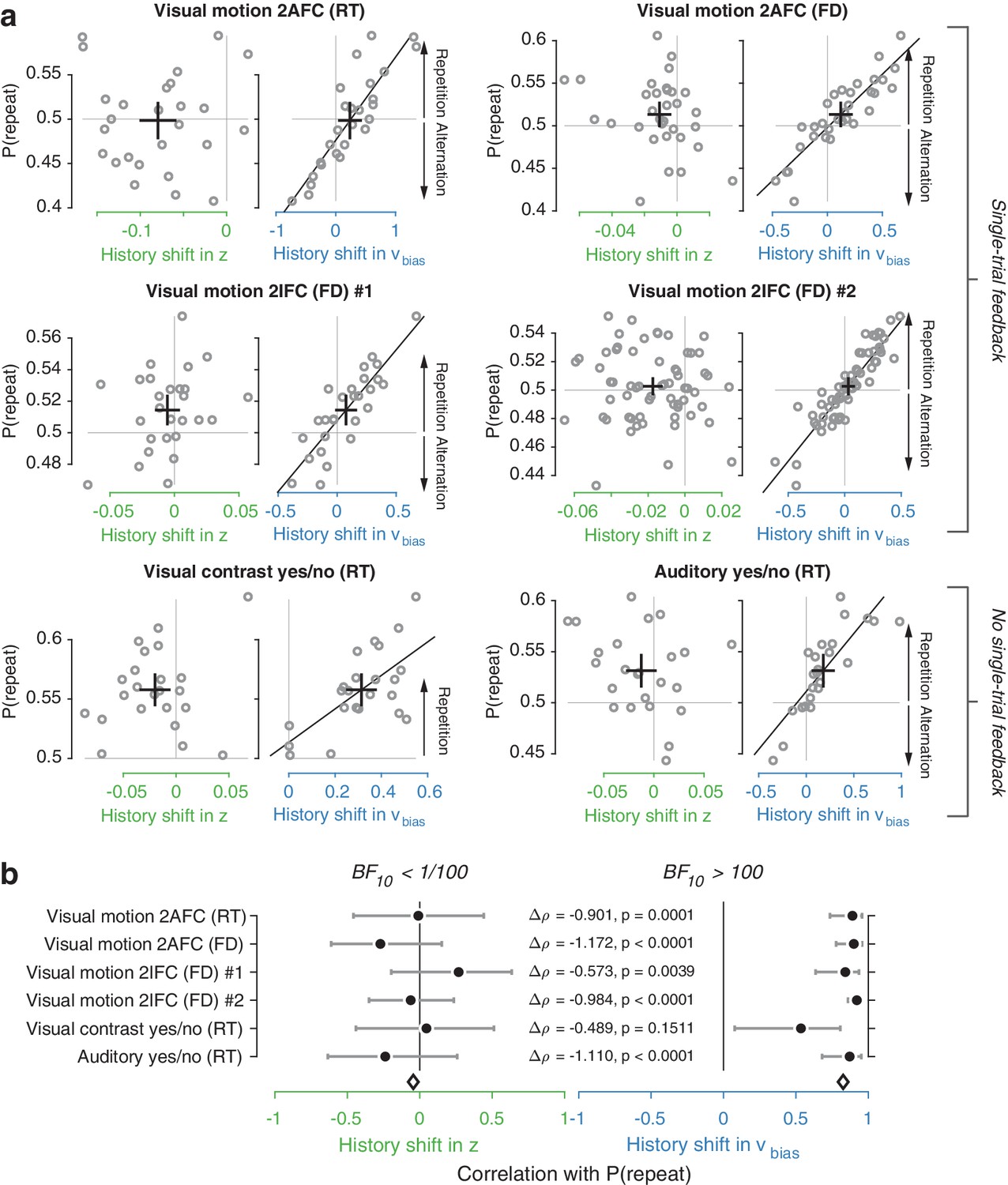
Individual choice history biases are explained by history-dependent changes in drift bias, not starting point.
(a) Relationship between individual choice repetition probabilities, P(repeat), and history shift in starting point (left column, green) and drift bias (right column, blue). Parameter estimates were obtained from a model in which both bias terms were allowed to vary with previous choice. Horizontal and vertical lines, unbiased references. Thick black crosses, group mean ± s.e.m. in both directions. Black lines: best fit of an orthogonal regression (only plotted for correlations significant at p<0.05). (b) Summary of the correlations (Spearman’s ρ) between individual choice repetition probability and the history shifts in starting point (green; left) and drift bias (blue; right). Error bars indicate the 95% confidence interval of the correlation coefficient. Δρ quantifies the degree to which the two DDM parameters are differentially able to predict individual choice repetition (p-values from Steiger’s test). The black diamond indicates the mean correlation coefficient across datasets. The Bayes factor (BF10) quantifies the relative evidence for the alternative over the null hypothesis, with values < 1 indicating evidence for the null hypothesis of no correlation, and >1 indicating evidence for a correlation.
Figure 4—figure supplement 1
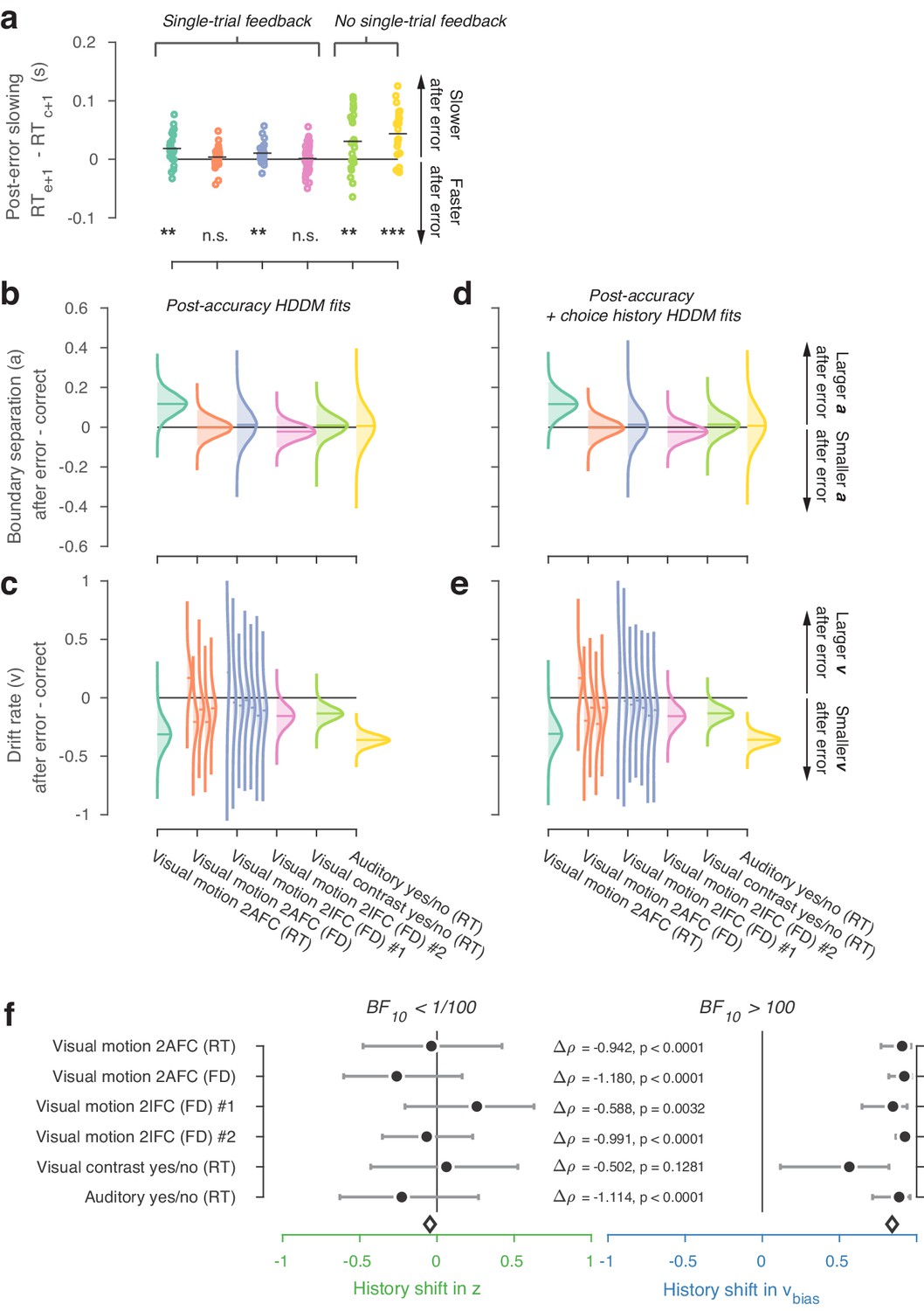
Post-error slowing.
(a) We computed post-error slowing as the difference in average RT after error and correct trials. In four of the six datasets, observers showed significant post-error slowing (permutation test against zero; ***p<0.001, **p<0.01, n.s. p>0.05). We then fit an HDDM model where the overall drift rate, as well as the boundary separation, were allowed to vary depending on the outcome (correct vs. error) of the previous trial. (b) Changes in boundary separation after error vs. correct trials. (c) Changes in drift rate after error vs. correct trials. For the two datasets with multiple levels of stimulus strength, the effect of previous error vs. correct on drift rate is shown separately for each discrete level of stimulus strength (weak to strong evidence from left to right; see also Materials and methods and Figure 3—figure supplement 2a). (d–e) as (b–c), but from a HDDM model where we simultaneously allowed choice history to affect starting point and drift bias, as well as previous accuracy to affect boundary separation and drift rate. Distributions were smoothed using kernel density fits. Shaded regions represent the 95% BCI, and white lines indicate the posterior mean. Errors were succeeded by a decrease in mean drift rate in most datasets and by an increased boundary separation in some datasets: both effects conspired to slow down decisions after an error. (f) Correlations between P(repeat) and history shifts in starting point and drift bias, from the model where previous accuracy was also allowed to affect boundary separation and drift rate.
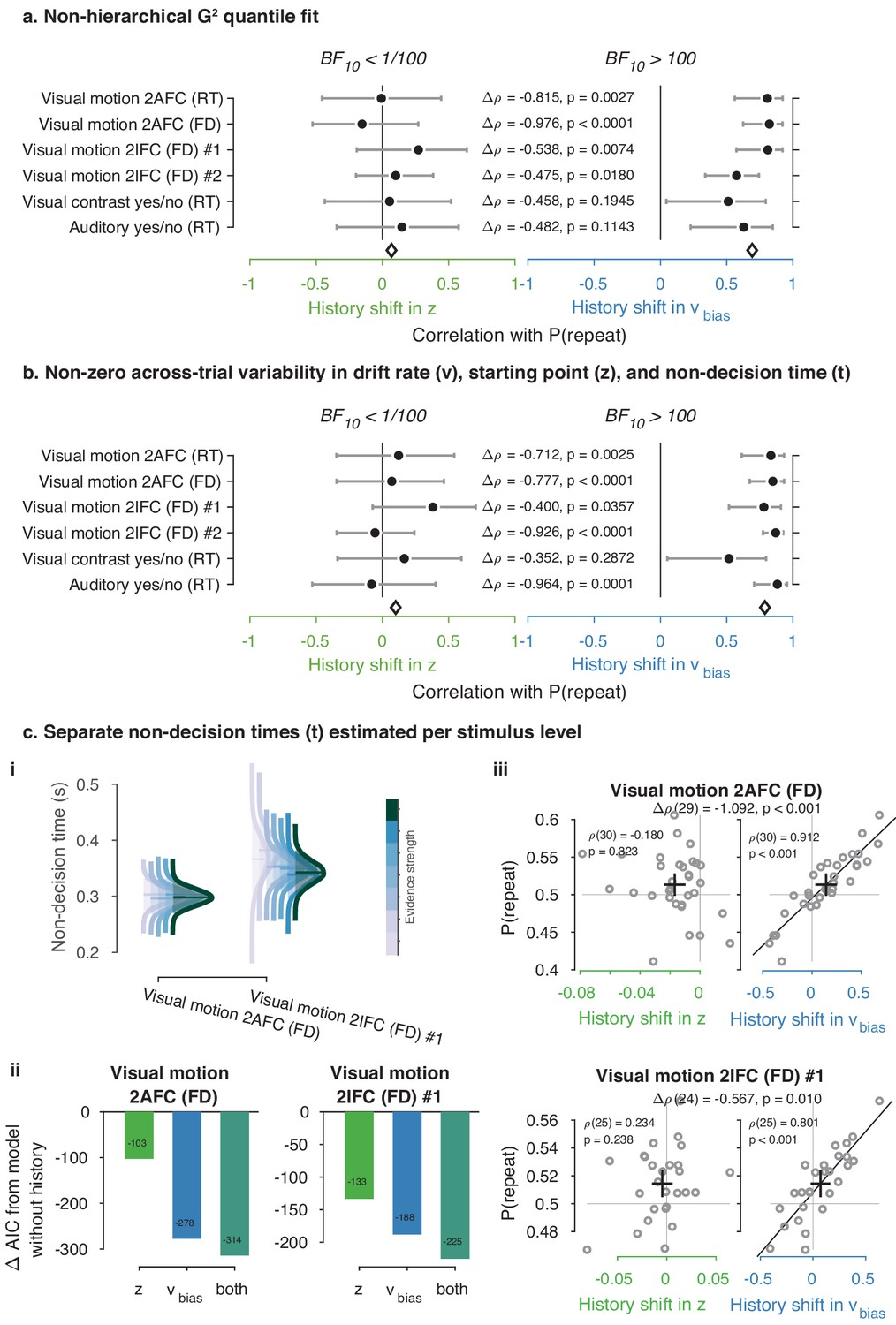
Figure 4—figure supplement 2
Control model fits.
(a) Summary figure based on non-hierarchical G2 fits (Ratcliff and Tuerlinckx, 2002). Rather than the full RT distribution, we fit each observers’ RT quantiles (0.1, 0.3, 0.5, 0.7, 0.9) and correlated history shifts in the DDM bias parameters to individual P(repeat), as in Figure 4. (b) Summary figure based on the full hierarchical model, where across-trial variability in non-decision time (st) was added as a free parameter. Like the across-trial variability in drift rate (sv) and starting point (sz), the st parameter was only estimated at the group level (Ratcliff and Childers, 2015). (c) Fits of the two datasets with multiple evidence strengths, allowing non-decision time to vary with these discrete levels (see Materials and methods). (i) Posterior distributions of group-level non-decision time for each level of evidence strength. (ii) Comparison between models accounting for choice history bias through a starting point, drift bias or both, while allowing for non-decision time to vary with levels of stimulus strength. (iii) Correlations between individual history shifts in starting point or drift bias and repetition probability, from a model where non-decision time was separately estimated per level of stimulus strength.
Figure 4—figure supplement 3
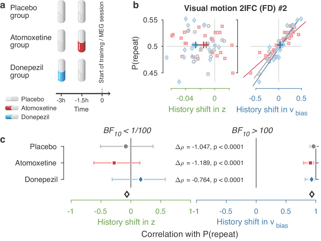
Same biasing mechanism under two pharmacological interventions.
(a) Participants in the MEG study were assigned to one of three pharmacological groups. At the start of each experimental session, they orally took 40 mg atomoxetine (Strattera), 5 mg donepezil (Aricept), or placebo. Since the time of peak plasma concentration is 3 hr for donepezil (Rogers and Friedhoff, 1998) and 1–2 hr for atomoxetine (Sauer et al., 2005), we used a placebo-controlled, double-blind, double-dummy design, entailing an identical number of pills at the same times before every session for all participants. Participants in the donepezil group took 5 mg of donepezil 3 hr, and placebo 1.5 hr before starting the experimental session. Participants in the atomoxetine group took placebo 3 hr, and 40 mg of atomoxetine 1.5 hr before the experimental session. Those in the placebo group took identical-looking sugar capsules both 3 and 1.5 hr before starting the session. This ensured that either drug reached its peak plasma concentration at the start of the experimental training. The drug doses were based on previous studies with healthy participants (Chamberlain et al., 2009; Rokem and Silver, 2010). Blood pressure and heart rate were measured and registered before subjects took their first and second pill. In the 3 hr before any MEG or training session, participants waited in a quiet room. In total, 19 people in the placebo, 22 in the atomoxetine, and 20 in the donepezil group completed the full study. (b, c) Choice history biases separately for each pharmacological group. Since we did not observe differences in choice history bias between these groups, we pooled all observers for the main analyses.
Figure 4—figure supplement 4
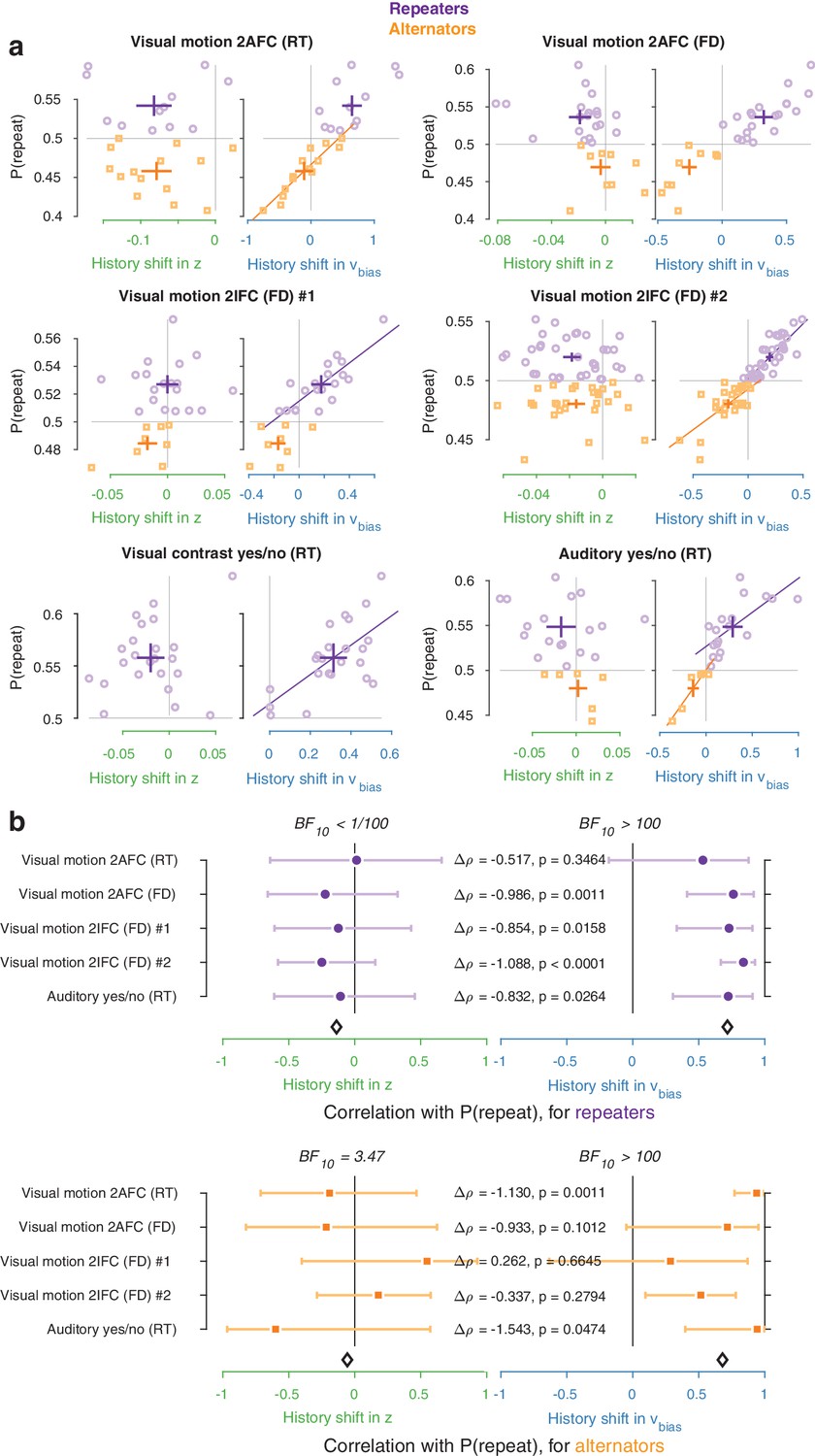
Repeaters vs. alternators.
(a) Correlations between individual history shifts in starting point or drift bias and repetition probability, fit separately for groups of ‘repeaters’ (P(repeat)>0.5) and ‘alternators’ (P(repeat)<0.5). (b) Summary of correlations (as in Figure 4c) separately for repeaters and alternators. Error bars indicate the 95% confidence interval of the correlation coefficient. Δρ quantifies the degree to which the two DDM parameters are differentially able to predict individual choice repetition, p-values from Steiger’s test. The black diamond indicates the mean correlation coefficient across datasets. In the Visual contrast yes/no RT dataset there were no alternators, so this dataset was excluded from the overview.
Figure 4—figure supplement 5
Group-level posterior distributions of history bias parameters.
History shift in (a) starting point and drift bias, as well as the effect of previous choice outcome on (b) starting point and drift bias, separately for each dataset. The posteriors were taken from the model where history-dependent z and vbias were fit simultaneously. Distributions were smoothed using kernel density fits. Shaded regions represent the 95% BCI, and white lines indicate the posterior mean. p-Values indicate the overlap with zero (a), or between the two conditions (b). (c) Repetition probability for five quantiles of the RT distribution, separately for each dataset (colors) and averaged across datasets (black). For those RTs < 600 ms, group-level behavior tended towards choice alternation.
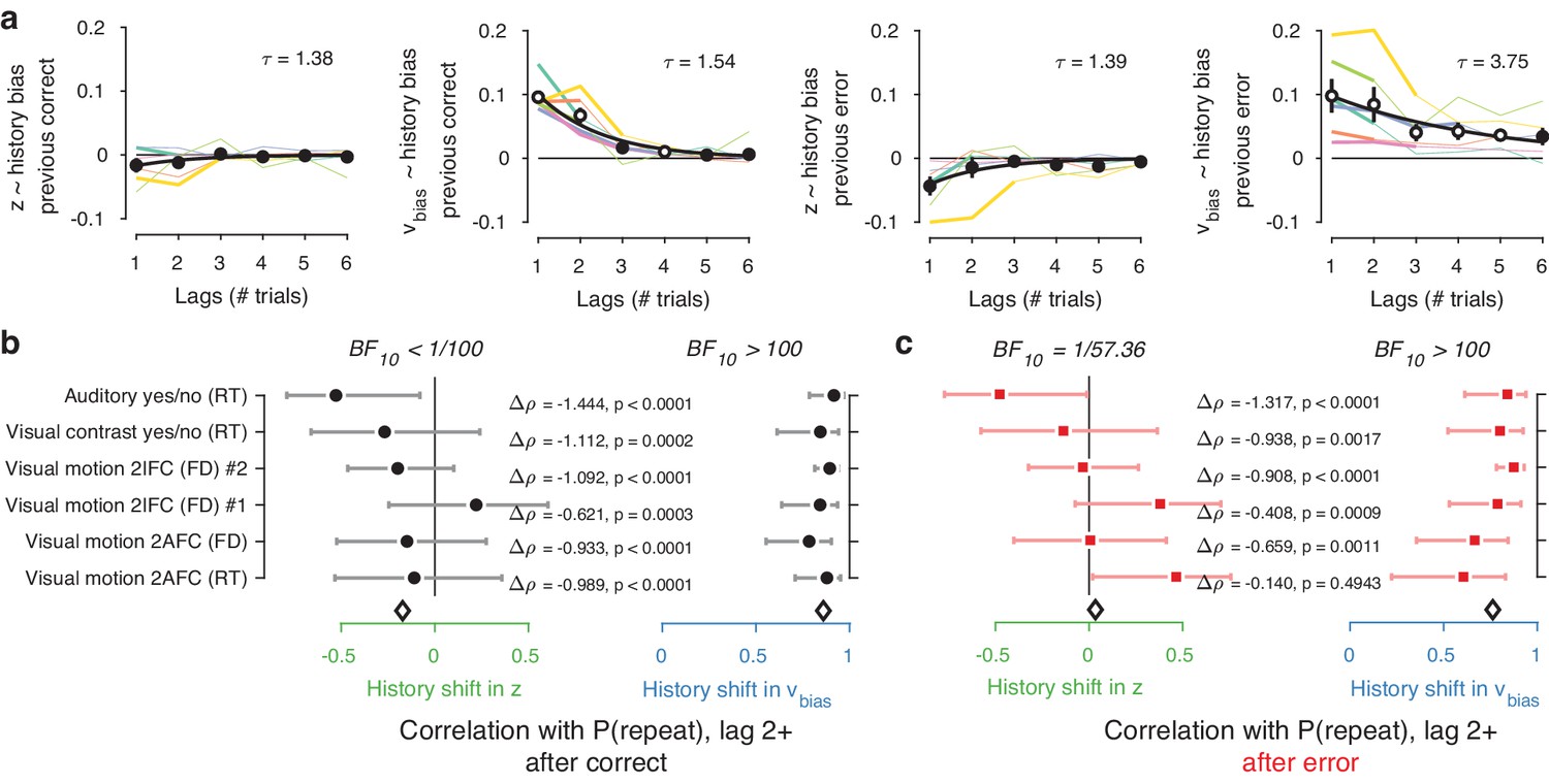
Figure 5

History shift in drift bias explains individual choice behavior after both error and correct decisions.
As in Figure 4, but separately following correct (black) and error (red) trials. Post-correct trials were randomly subsampled to match the trial numbers of post-error trials. (a) Relationship between repetition probability and history shifts in starting point and drift bias, separately computed for trials following correct (black circles) and error (red squares) responses. (b) Summary of correlations (as in Figure 4c) for trials following a correct response. Error bars indicate the 95% confidence interval of the correlation coefficient. (c) Summary of correlations (as in Figure 4c) for trials following an error response. (d) Difference in correlation coefficient between post-correct and post-error trials, per dataset and parameter. Δρ quantifies the degree to which the two DDM parameters are differentially able to predict individual choice repetition (p-values from Steiger’s test). The black diamond indicates the mean correlation coefficient across datasets. The Bayes factor (BF10) quantifies the relative evidence for the alternative over the null hypothesis, with values < 1 indicating evidence for the null hypothesis of no correlation, and >1 indicating evidence for a correlation.
Figure 6 with 1 supplement
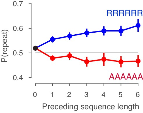
Choice history affects drift bias over multiple trials.
(a) History kernels, indicating different parameters’ tendency to go in the direction of each individual’s history bias (i.e. sign-flipping the parameter estimates for observers with P(repeat)<0.5). For each dataset, regression weights from the best-fitting model (lowest AIC, Figure 6—figure supplement 1) are shown in thicker lines; thin lines show the weights from the largest model we fit. Black errorbars show the mean ± s.e.m. across models, with white markers indicating timepoints at which the weights are significantly different from zero across datasets (p<0.05, FDR corrected). Black lines show an exponential fit to the average. (b) Correlations between individual P(repeat) and regression weights, as in Figure 5b–c. Regression weights for the history shift in starting point and drift bias were averaged from lag two until each dataset’s best-fitting lag. P(repeat) was corrected for expected repetition at longer lags given individual repetition, and averaged from lag two to each dataset’s best-fitting lag. Δρ quantifies the degree to which the two DDM parameters are differentially able to predict individual choice repetition (p-values from Steiger’s test). The black diamond indicates the mean correlation coefficient across datasets. The Bayes factor (BF10) quantifies the relative evidence for the alternative over the null hypothesis, with values < 1 indicating evidence for the null hypothesis of no correlation, and >1 indicating evidence for a correlation.
Figure 6—figure supplement 1
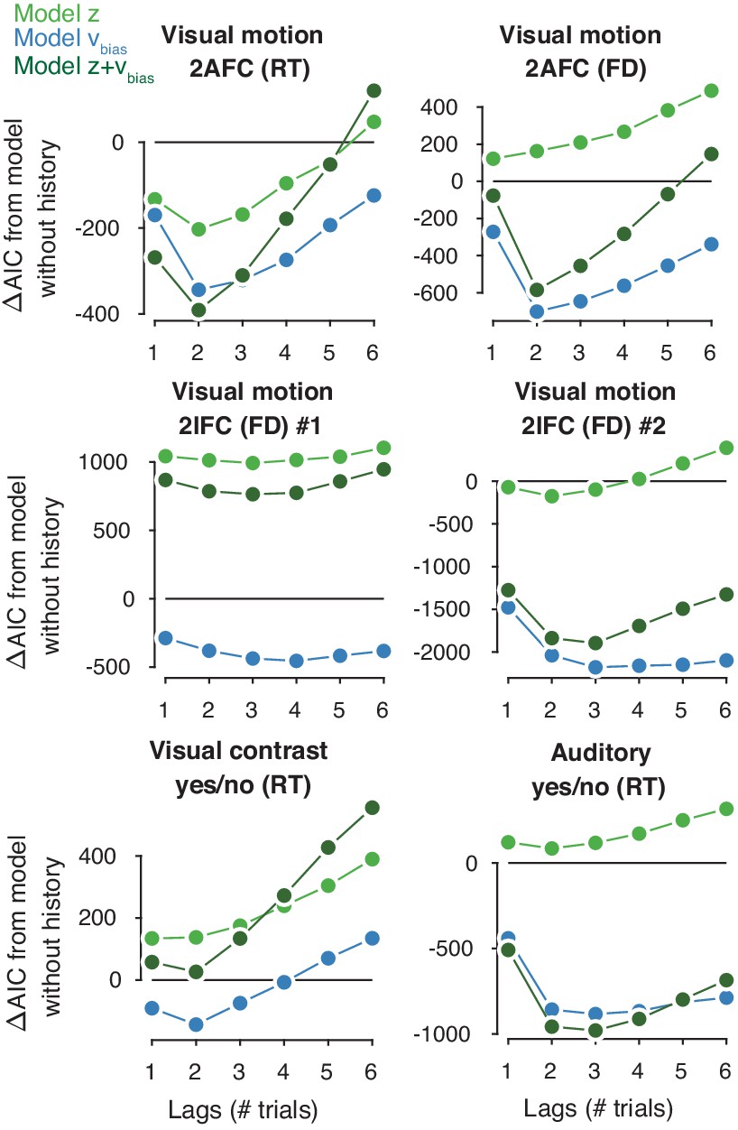
Contribution of previous choices to current drift and starting point bias as function of lag.
Model comparison (ΔAIC from a baseline model without history) between models where previous correct and incorrect choices affected only starting point (light green squares), only drift bias (blue diamonds), or both (blue-green circles), up to six past trials. The best-fitting model is indicated by a black outline.
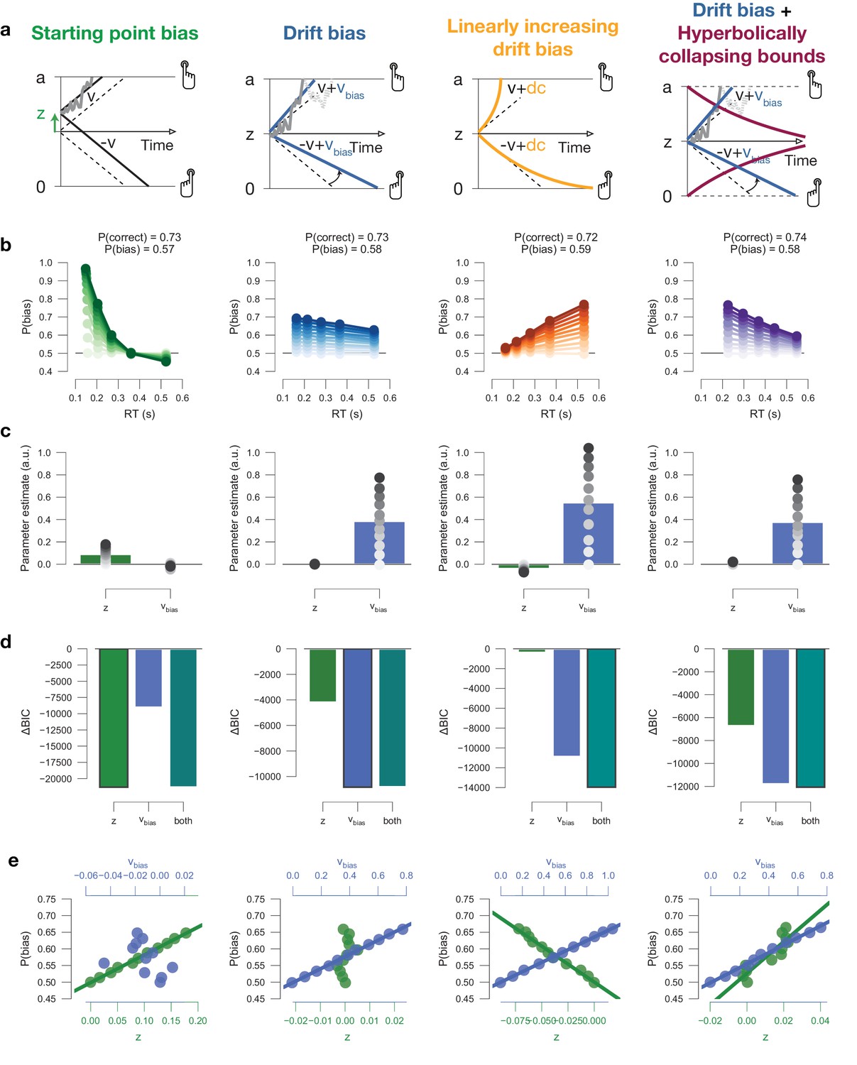
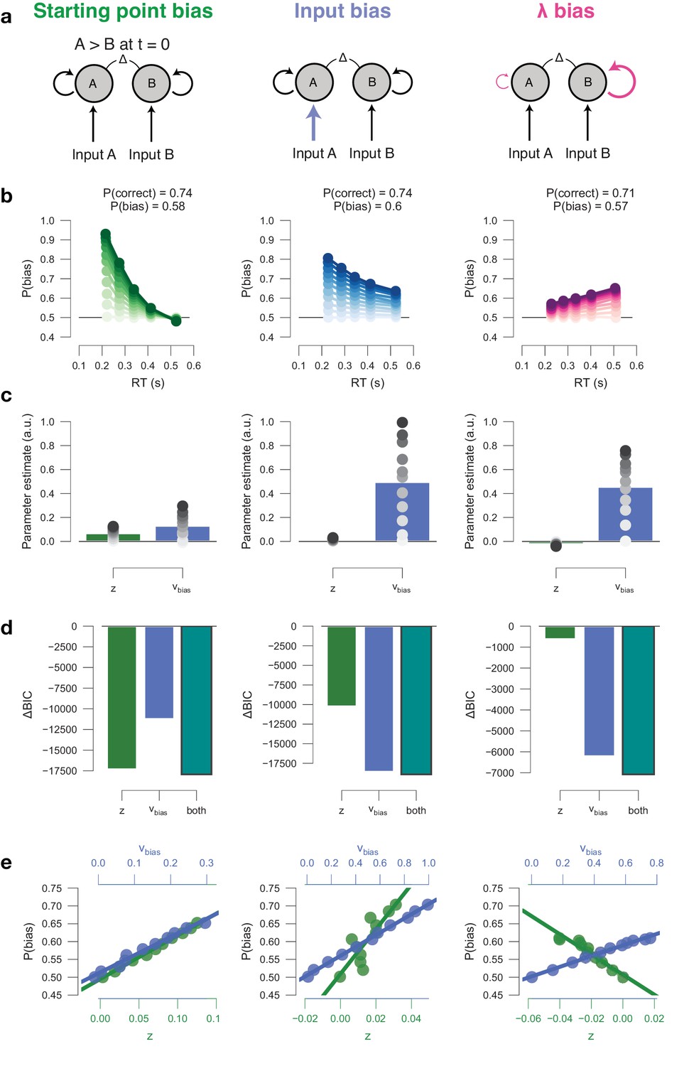
Figure 7 with 3 supplements
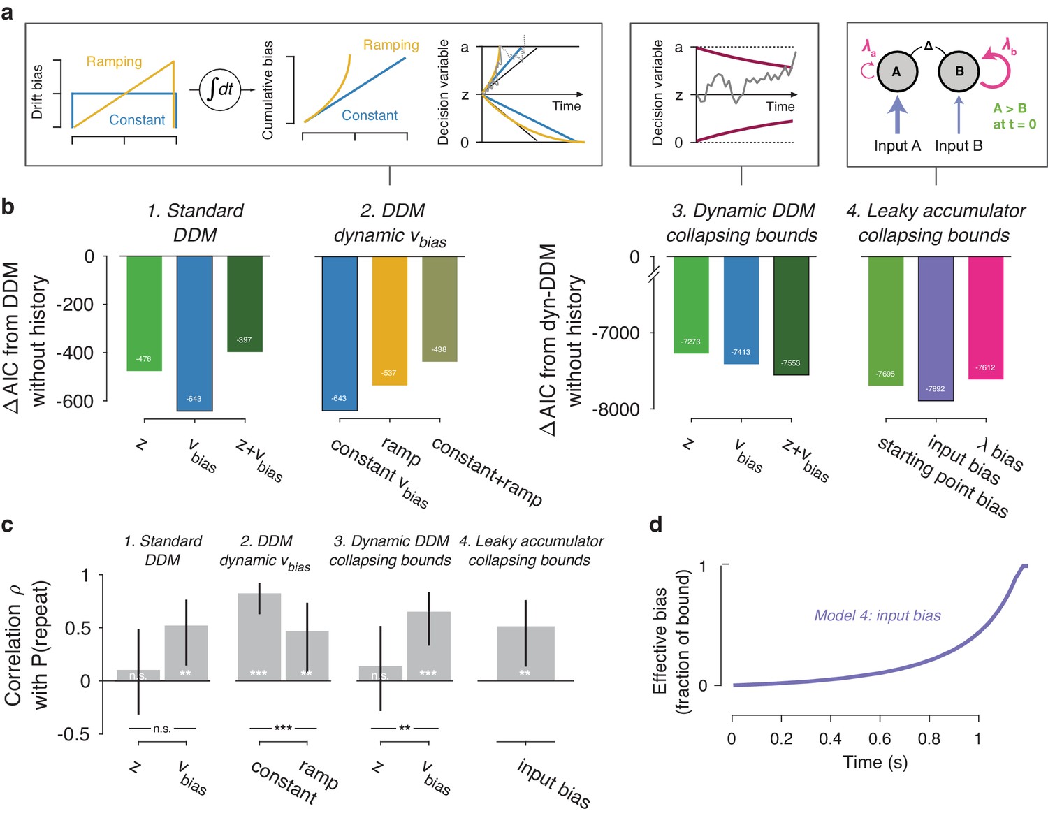
Extended dynamic models of biased evidence accumulation.
(a) Model schematics. In the third panel from the left, the stimulus-dependent mean drift is shown in black, overlaid by the biased mean drift in color (as in Figure 1a,b). (b) AIC values for each history-dependent model, as compared to a standard (left) or dynamic (right) DDM without history. The winning model (lowest AIC value) within each model class is shown with a black outline. (c) Correlation (Spearman’s ρ) of parameter estimates with individual repetition behavior, as in Figure 4b. Error bars, 95% confidence interval. ***p<0.0001, **p<0.01, n.s. p>0.05. (d) Within-trial time courses of effective bias (cumulative bias as a fraction of the decision bound) for the winning leaky accumulator model. Effective bias time courses are indistinguishable between both dynamical regimes (λ < 0 and λ > 0) and are averaged here.
Figure 7—figure supplement 1
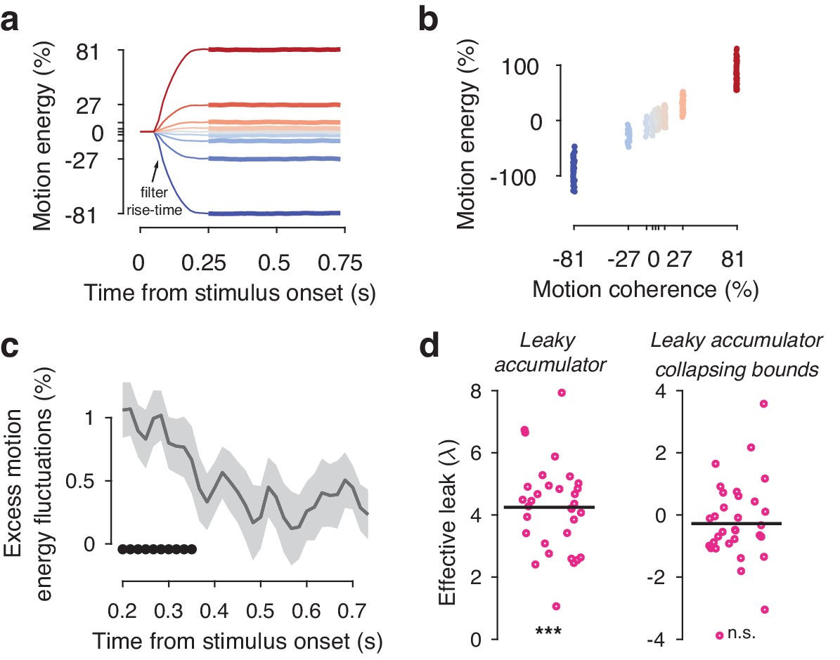
Motion energy filtering, psychophysical kernels and the effective time-constant of evidence integration.
(a) Within each generative coherence level, the average motion energy traces were rescaled to express motion energy in % coherence. The initial 200 ms of the trial fall within the rise-time of the spatiotemporal motion energy filter. (b) The average motion energy is a linear function of coherence, with substantial trial-by-trial fluctuations that arise from the stochastically generated noise dots. Note that while we previously used motion energy filtering on the dot coordinates in the Visual motion 2IFC (FD) #1 dataset (Urai et al., 2017), the large stimulus display in that study resulted in most noise fluctuations being averaged out over space. This resulted in only small trial-by-trial differences in the effective decision-relevant input). (c) Psychophysical kernels, indicating the effect of fluctuations in motion energy (using the three weakest coherence levels) on observers’ choice over time. Shaded errorbars indicate group s.e.m., black dots show significant (p<0.05, FDR-corrected) group-level deviations from zero. (d) Individual effective leak parameters, estimated from an leaky accumulator model either without (left) or with (right) collapsing. A positive λ indicates that the accumulators accelerate towards the decision bound, depending on the value of the decision variable. When including a collapsing bound in the model, which captures an overall urgency in the decision process, overall effective leak biases are no longer significantly different from zero. ***p<0.001, **p<0.01, n.s. p>0.05, permutation test against zero.
Figure 7—figure supplement 2
Leaky accumulator model simulators.
To match the empirical data (Figure 7—figure supplement 1d), we choose the overall leak parameter to be > 0, producing a primacy effect through self-excitatory accumulators, whereby evidence early on in the trials has a stronger leverage on choice. We verified that the same conclusions hold for (data not shown). All simulations included collapsing bounds. (a) Model schematics. Left to right: (i) The effect of a biased starting point on choice declines rapidly with elapsed time, as the decision variable is increasingly governed by the input. (ii) The effect of biased input to the accumulation stage within the leaky accumulator model is uniquely captured by drift bias within the DDM. Also, the effect input bias on choice increases with elapsed time, as the decision variable is increasingly governed by the bias. (iii) The effect of biased leak of the accumulators (henceforth termed ‘ bias’) on choice increases with elapsed time, as the decision variable is increasingly governed by the bias. (b) Conditional bias functions, for synthetic individuals with increasing bias magnitude (indicated by color intensity). (c) Parameter estimates of a hybrid HDDM (with both starting point and drift bias) fit on simulated data. (d) Model comparison from a baseline model without history. The best-fitting model is indicated with a black outline. (e) Correlations between P(bias) of each synthetic individual, and their respective parameter estimates for both starting point and drift bias. It noteworthy that bias in the leaky accumulator model predicts the strongest choice bias for long RTs, while both DDM starting point and drift bias predict the strongest choice bias for short RTs. This implies that if a major source of choice bias in any dataset is due to a leak bias, the DDM is not going to be able to easily account for this. Our simulations show that the best-fitting DDM such data shows: (i) a drift bias, in order to explain the choice bias for relatively long RTs, and (ii) a starting point of opposite sign, in order to push down the expected choice bias for relatively short RTs. Indeed, these opposing effects of starting point and drift bias can be observed in the bars in (h), and are present in some of the datasets used here (Figure 4—figure supplement 5a). The present simulation results suggest that even stronger choice repetition (or alternation) effects as measured here would give rise to opposite effects on starting point and drift bias in DDM fits.
Figure 7—figure supplement 3
Drift diffusion model simulations.
(a) Model schematics. (b) Conditional bias functions, for synthetic individuals with increasing bias magnitude (indicated by color intensity). (c) Parameter estimates of a hybrid HDDM (with both starting point and drift bias) fit on simulated data. (d) Model comparison from a baseline model without history. The best-fitting model (lowest BIC) is indicated by a black outline. (e) Correlations between P(bias) of each synthetic individual, and their respective parameter estimates for both starting point and drift bias.
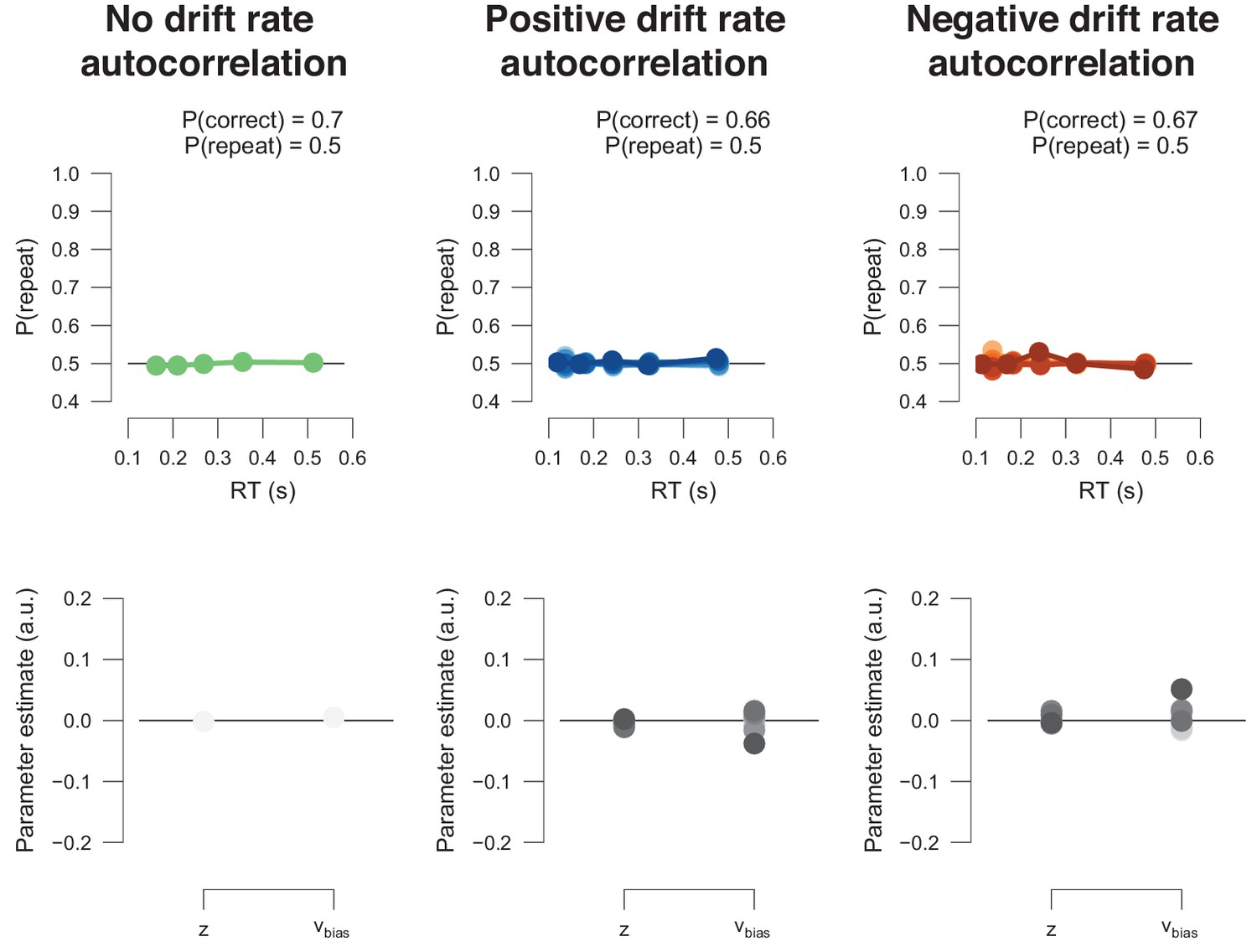
Author response image 1

Author response image 2
Author response image 3
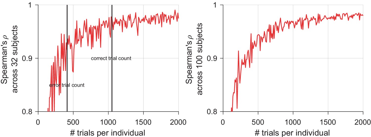
Author response image 4
Additional files
-
Transparent reporting form
- https://doi.org/10.7554/eLife.46331.020
Download links
A two-part list of links to download the article, or parts of the article, in various formats.
Downloads (link to download the article as PDF)
Open citations (links to open the citations from this article in various online reference manager services)
Cite this article (links to download the citations from this article in formats compatible with various reference manager tools)
Choice history biases subsequent evidence accumulation
eLife 8:e46331.
https://doi.org/10.7554/eLife.46331


