Resolving multisensory and attentional influences across cortical depth in sensory cortices
Figures
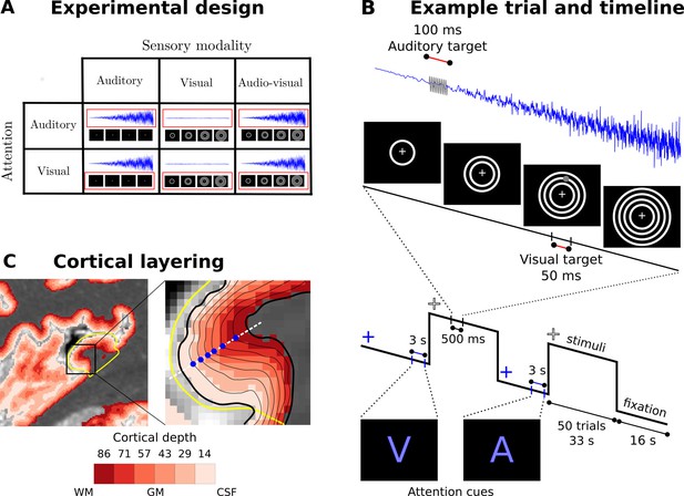
Experimental design, timeline and cortical layering.
(A) Experimental design: Participants were presented with auditory, visual and audiovisual looming stimuli under auditory and visual attention. (B) Example trial and timeline: Participants were presented with brief auditory, visual or audiovisual looming stimuli in 33 s blocks interleaved with 16 s fixation. At the beginning of each block, a cue indicated whether the auditory or visual modality needed to be attended. Brief visual and auditory targets (grey) were interspersed in the looming activation blocks. Participants were instructed to respond to the targets in the attended and ignore the targets in the unattended sensory modality. (C) Cortical layering: Left: A parasagittal section of a high resolution T1 map is shown with a colour coded laminar label for each voxel (voxel size: (0.4 mm)3). The primary auditory cortex is circled in yellow. Right: The cortical sheet is defined by the pial and white matter surfaces (thick black solid lines). Six additional surfaces (thin black solid lines) were determined at different cortical depths. Data were mapped onto those surfaces by sampling (blue dots) radially along the normal (white dashed line) to the mid-cortical depth surface (not shown here). WM: white matter, GM: grey matter, CSF: cerebrospinal fluid.
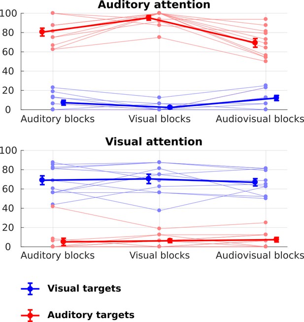
Behavioural results.
Percentage of responses to auditory (red) and visual (blue) targets in auditory, visual and audiovisual blocks (along the x-axis) and under auditory (top panel) and visual (bottom panel) attention. Thick lines represent group means + /- SEM and each thin line represents a participant. Responses to visual targets under auditory attention and responses to auditory targets under visual attention are false alarms (and vice versa for visual attention).
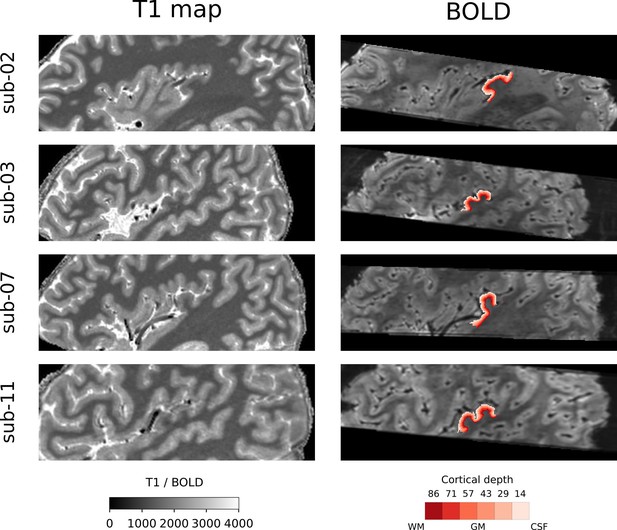
Segmentation and coregistration.
Sagittal section of T1 structural images (left), the corresponding coregistered mean EPI images of four representative participants. The definition of the six laminae is overlaid in A1.
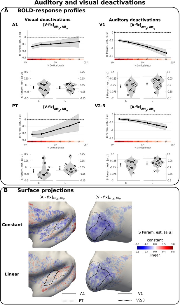
Auditory and visual deactivations.
(A) BOLD response profiles: Rows 1 and 3: The BOLD response (i.e. B parameters, across subjects’ mean ± SEM) for visual and auditory looming stimuli averaged over auditory and visual attention in A1, PT, V1, V2/3 is shown as a function of percentage cortical depth. WM: white matter; GM: grey matter; CSF: cerebrospinal fluid. Percentage cortical depth is indicated by the small numbers and colour coded in red. Rows 2 and 4: Across subjects’ mean (± SEM) and violin plot of the participants’ shape parameter estimates that characterize the mean (C: constant) and linear increase (L: linear) of the laminar BOLD response profile. n = 11. (B) Surface projections: Across subject’ mean of the ‘constant’ (row i) and ‘linear’ increase (row ii) shape parameter estimates of the laminar BOLD response profile for auditory and visual looming stimuli (averaged over auditory and visual attention) are projected on an inflated group mean surface to show auditory and visual regions of the left hemisphere. A1 and V1 are delineated by black solid lines, PT and V2/3 by dashed lines. For visualization purposes only: i. surface projections were smoothed (FWHM = 1.5 mm); ii. values are also presented for vertices for which data were not available from all subjects and which were therefore not included in our formal statistical analysis. Grey areas denote vertices with no available data for any subject.
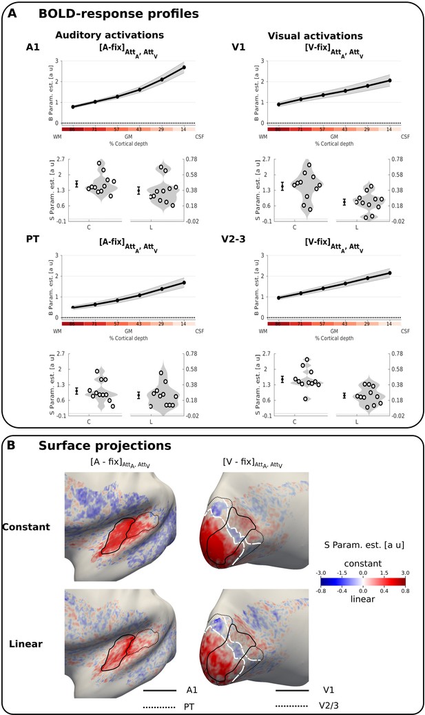
Auditory and visual activations.
(A) BOLD response profiles: Row 1 and 3: The BOLD response (i.e. B parameters, across subjects’ mean ± SEM) for auditory and visual activations induced by looming stimuli averaged over auditory and visual attention in A1, PT, V1, V2/3 is shown as a function of percentage cortical depth. WM: white matter; GM: grey matter; CSF: cerebrospinal fluid. Percentage cortical depth is indicated by the small numbers and colour coded in red. Rows 2 and 4: Across subjects’ mean (± SEM) and violin plot of the participants’ shape parameter estimates that characterize the mean (C: constant) and linear increase (L: linear) of the laminar BOLD response profile. n = 11. (B) Surface projections: Across subject’ mean of the ‘constant’ (row i) and ‘linear’ increase (row ii) shape parameter estimates of the laminar BOLD response profile for auditory and visual looming stimuli (averaged over auditory and visual attention) are projected on an inflated group mean surface to show auditory and visual regions of the left hemisphere. A1 and V1 are delineated by black solid lines, PT and V2/3 by dashed lines. For visualization purposes only: i. borders between visual-induced activations and deactivations (white dashed lines) were defined based on visual inspection; ii. surface projections were smoothed (FWHM = 1.5 mm); iii. values are also presented for vertices for which data were not available from all subjects and which were therefore not included in our formal statistical analysis. Grey areas denote vertices with no available data for any subject.
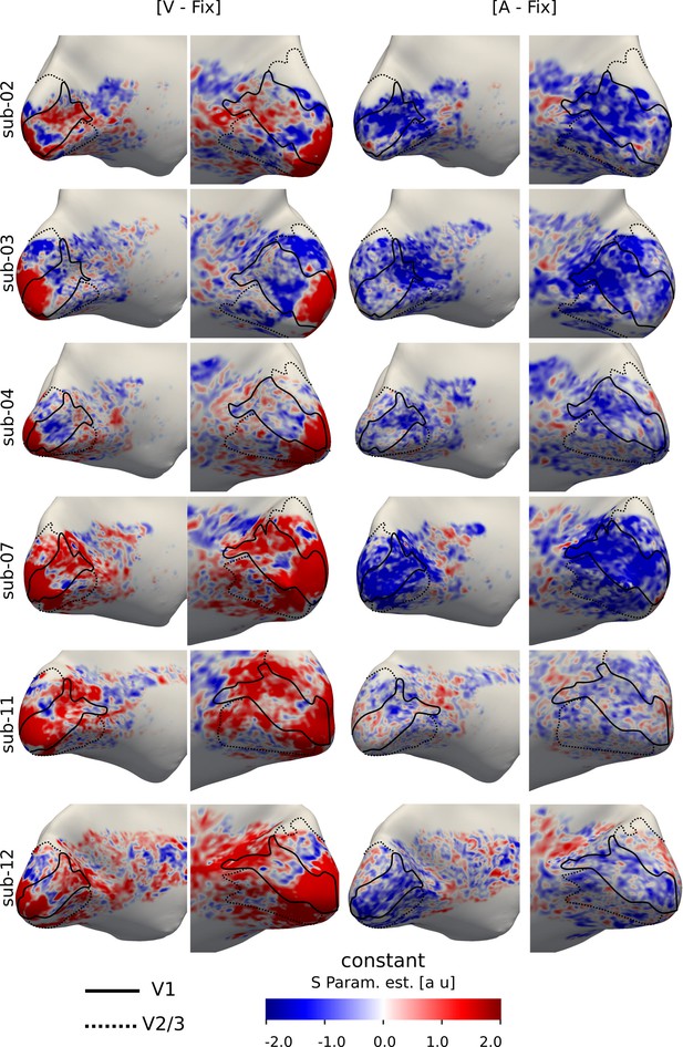
Auditory and visual responses in visual areas.
Surface projection for individual subjects: Within subject ‘constant’ shape parameter estimates of the laminar BOLD response profile for visual (column i and ii) and auditory (column iii and iv) stimuli are projected on each subject’s inflated surface to show visual regions of the left (column i and iii) and right (column ii and iv) hemisphere. V1 and V2/3 are delineated by black solid and dashed lines respectively. For visualization purposes only, surface projections were smoothed (FWHM = 1.5 mm). Grey areas denote vertices with no available data.
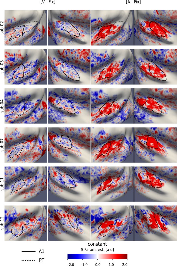
Auditory and visual responses in auditory areas.
Surface projection for individual subjects: Within subject ‘constant’ shape parameter estimates of the laminar BOLD response profile for visual (column i and ii) and auditory (column iii and iv) are projected on each subject’s inflated surface to show visual regions of the left (column i and iii) and right (column ii and iv) hemisphere. A1 and PT are delineated by black solid and dashed lines, respectively. For visualization purposes only, surface projections were smoothed (FWHM = 1.5 mm). Grey areas denote vertices with no available data.
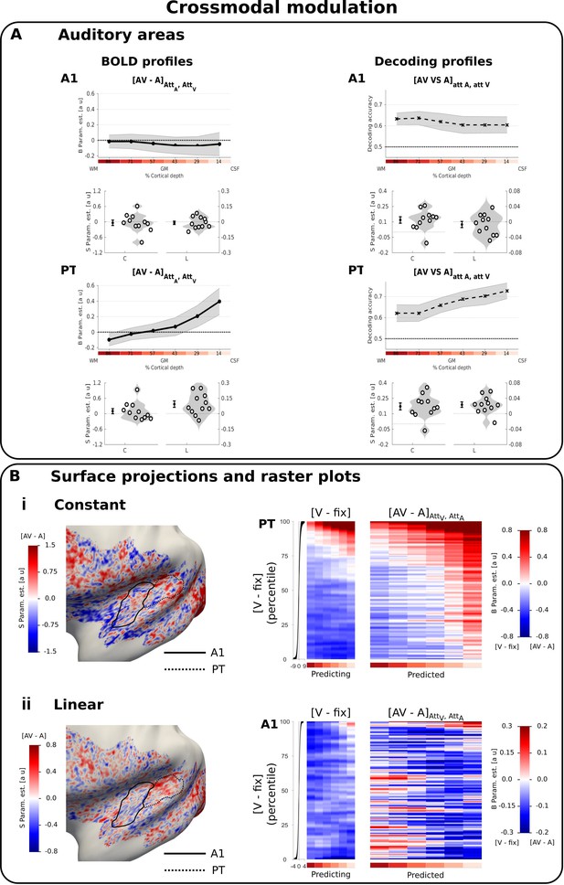
Cross-modal modulation in auditory areas.
(A) Laminar profiles: Rows 1 and 3: The BOLD response (solid line; column 1 and 3) and decoding accuracy (dashed line; columns 2 and 4) (across subjects’ mean ± SEM) for [AV-A] in A1 and PT is shown as a function of percentage cortical depth pooled (i.e. averaged) over auditory and visual attention. WM: white matter, GM: grey matter, CSF: cerebrospinal fluid. Percentage cortical depth is indicated by the small numbers and colour coded in red. Rows 2 and 4: Across subjects’ mean (± SEM) and violin plot of participants’ shape parameter estimates that characterize the mean (C: constant) and linear increase (L: linear) of the laminar BOLD response and decoding accuracy profiles. n = 11. (B) Surface projections and raster plots: Left: Across subject’ mean of the ‘constant’ (row i) and ‘linear increase’ (row ii) shape parameter estimates of the laminar BOLD response profile for [AV-A] (averaged over auditory and visual attention) are projected on an inflated group mean surface to show auditory regions of the left hemisphere. A1 and PT are delineated by black solid and dashed lines. For visualization purposes only: i. surface projections were smoothed (FWHM = 1.5 mm); ii. values are also presented for vertices for which data were not available from all subjects and which were therefore not included in our formal statistical analysis. Grey areas denote vertices with no available data for any subject. Right: Row i. PT: The raster plot illustrates the statistical relationship between the ‘constant’ shape parameters for the visual evoked response [V-Fix]AttA, AttV and the crossmodal modulation [AV-A]AttA, AttV in PT. Each raster plot shows the laminar profiles (colour coded along abscissa) of the vertices for the ‘predicting contrast’ [V-Fix] and of the ‘predicted contrast’ [AV-A]. The laminar profiles of the vertices were sorted along the ordinate according to the value of the ‘constant’ shape parameter for [V-Fix]. The raster plot shows that the laminar profile of a vertex for [V-Fix] can predict its laminar profile for [AV-A]: PT vertices with less deactivations across laminae for [V-Fix] are associated with greater crossmodal enhancement [AV-A]. Row ii. The raster plot illustrates the statistical relationship between the ‘linear slope’ shape parameters for the visual evoked response [V-Fix]AttA, AttV and the crossmodal modulation [AV-A] in A1. Each raster plot shows the laminar profiles (colour coded along abscissa) of the vertices for the ‘predicting contrast’ [V-Fix] and of the ‘predicted contrast’ [AV-A]. The laminar profiles of the vertices are sorted along the ordinate according to the value of the ‘linear’ shape parameter for [V-Fix]. A1 vertices with less deactivations in deeper laminae for [V-Fix] are associated with greater crossmodal enhancement [AV-A] in deeper laminae. To enable averaging the raster plots across participants, the vertices were binned after sorting (number of bins for A1: 10100, number of bins for PT: 6800). For visualization purposes all raster plots were smoothed along the vertical axis (FWHM = 1% of the number of data bins). The subplot (i.e. black line) to the left of the raster plots shows the across subjects’ mean value (+ /- STD) of the shape parameters (i.e. i. constant, ii, linear) of the sorting contrast. n = 11.
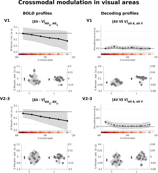
Cross-modal modulation in visual areas.
Laminar profiles: Rows 1 and 3: The BOLD response (solid line; column 1 and 3) and decoding accuracy (dashed line; columns 2 and 4) (across subjects’ mean ± SEM) for [AV-A] in V1 and V2/3 is shown as a function of percentage cortical depth pooled (i.e. averaged) over auditory and visual attention. WM: white matter, GM: grey matter, CSF: cerebrospinal fluid. Percentage cortical depth is indicated by the small numbers and colour coded in red. Rows 2 and 4: Across subjects’ mean (± SEM) and violin plot of participants’ shape parameter estimates that characterize the mean (C: constant) and linear increase (L: linear) of the laminar BOLD response and decoding accuracy profiles. n = 11.
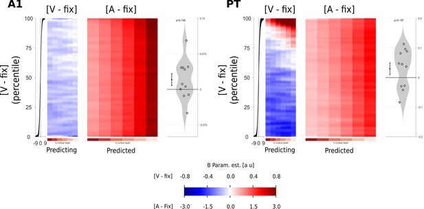
Raster plots for auditory induced activations and visual induced deactivations in auditory areas.
The raster plots illustrate the statistical relationship between the ‘constant’ shape parameters for the visual evoked response [V-Fix]AttA, AttV and auditory evoked response [A-Fix]AttA, AttV in A1 (left) and PT (right). Each raster plot shows the laminar profiles (colour coded along abscissa) of the vertices for the ‘predicting contrast’ [V-Fix] and of the ‘predicted contrast’ [A-Fix]. The vertex profiles were sorted along the ordinate according to the value of the ‘constant’ shape parameter for [V-Fix]. The raster plot shows that the laminar profile of a vertex for [V-Fix] cannot predict its laminar profile for [A-Fix]. To enable averaging the raster plots across participants, the vertices were binned after sorting (number of bins for A1: 10100, number of bins for PT: 6800). For visualization purposes, all raster plots were smoothed along the vertical axis (FWHM = 1% of the number of data bins). The subplot (i.e. black line) to the left of the raster plots shows the across subjects’ mean value (+ /- STD) of the shape parameters (i.e. i. constant, ii, linear) of the sorting contrast. The violin plot show the distribution across subject of beta values for ‘a’ in the regression model [A-Fix]=a [V-FIX] + b. n = 11.
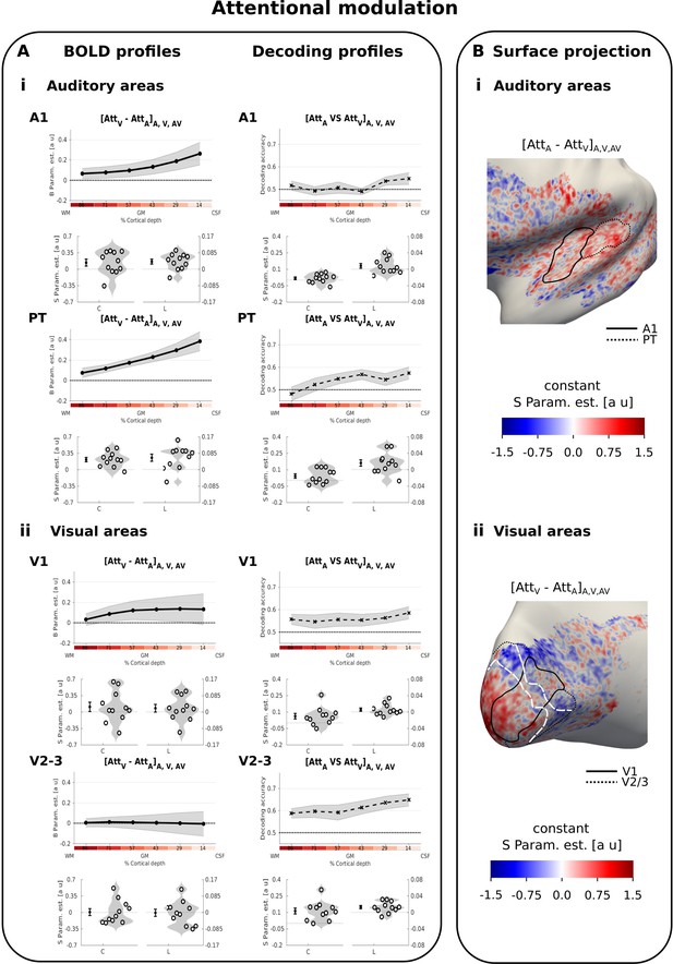
Attentional modulation.
(A) Laminar profiles: Rows 1, 3, 5, 7: The BOLD response (solid line; columns 1 and 3) and decoding accuracy (dashed line; columns 2 and 4) (across subjects’ mean ± SEM) for attentional modulation (i: top - [AttA-AttV] in A1 and PT; ii: bottom - [AttV-AttA] in V1 and V2/3) is shown as a function of percentage cortical depth pooled (i.e. averaged) over auditory, visual and audiovisual looming stimuli. WM: white matter, GM: grey matter, CSF: cerebrospinal fluid. Percentage cortical depth is indicated by the small numbers and colour coded in red. Rows 2, 4, 6, 8: Across subjects’ mean (± SEM) and violin plot of the participants’ shape parameter estimates that characterize the mean (C: constant) and linear increase (L: linear) of the laminar BOLD response and decoding accuracy profiles. n = 11. B. Surface projections: Across subject’ mean of the ‘constant’ shape parameter estimates for attentional modulation [AttA-AttV]A,V, AV in A1 and PT (i: top) and in V1 and V2/3 (ii: bottom) are projected on an inflated group mean surface of the left hemisphere. A1 and V1 are delineated by black solid lines. PT and V2/3 are delineated by dashed lines. For visualization purposes only: i. surface projections were smoothed (FWHM = 1.5 mm); ii. values are also presented for vertices for which data were not available from all subjects and which were therefore not included in our formal statistical analysis; iii borders between visual-induced activations and deactivations (white dashed lines on the right) are reported here from Figure 2B. Grey areas denote vertices with no available data for any subject.
Tables
Auditory and visual deactivations.
| Linear or constant | Constant | Linear | ||||||
|---|---|---|---|---|---|---|---|---|
| [V-fix]Att_A, Att_V | Mean(A1, PT) | F(2,40) = 9.280 | p<0.001 | t(10)=−2.460 | p=0.017* | F(1,20) = 2.083 | p=0.164 | |
| A1 | t(10)=−2.077 | p=0.032* | ||||||
| PT | t(10)=−2.042 | p=0.034* | ||||||
| [A-fix]Att_A, Att_V | mean(V1, V23) | F(2,40) = 58.615 | p<0.001 | t(10)=−5.547 | p<0.001* | F(1,20) = 22.433 | p<0.001 | |
| V1 | t(10)=−6.538 | p<0.001* | t(10)=−5.080 | p<0.001 | ||||
| V2-3 | t(10)=−4.305 | p<0.001* | t(10)=−4.142 | p=0.002 | ||||
-
*indicates p-values based on a one-sided t-test based on a priori hypotheses. p-values<0.05 are indicated in bold. n = 11
Using 2 (shape parameter: constant, linear) x 2 (ROI: primary, non-primary) linear mixed effects models, we performed the following statistical comparisons in a 'step down procedure':
-
1. Two-dimensional F-test assessing whether the constant or linear parameter (e.g. each averaged across ROIs in auditory resp. visual cortices), was significantly different from zero (dark grey),
2. If this two-dimensional F-test was significant, we computed one dimensional F-tests separately for the constant and the linear parameters (again averaged across auditory resp. visual ROIs) (light grey),
-
3. If the one dimensional F-test was significant, we computed follow-up t-tests separately for each of the two ROIs (white).
Effects of the cross-modal modulation on the laminar BOLD response and decoding accuracy profiles in auditory areas.
| A) BOLD profile | ||||||||
|---|---|---|---|---|---|---|---|---|
| linear or constant | constant | linear | ||||||
| [AV - A]Att_A, Att_V | mean(A1, PT) | F(2,40) = 0.196 | p=0.823 | |||||
| B) Decoding profile | ||||||||
| linear or constant | constant | linear | ||||||
| [AV VS A]att A, att V | mean(A1, PT) | F(2,40) = 34.946 | p<0.001 | F(1,20) = 21.966 | p<0.001 | F(1,20) = 1.850 | p=0.189 | |
| A1 | t(10)=3.867 | p=0.003 | ||||||
| PT | t(10)=4.992 | p<0.001 | ||||||
-
Using 2 (shape parameter: constant, linear) x 2 (ROI: primary, non-primary) linear mixed effects models, we performed the following statistical comparisons in a 'step down procedure':
1. Two-dimensional F-test assessing whether the constant or linear parameter (e.g. each averaged across ROIs in auditory resp. visual cortices), was significantly different from zero (dark grey),
-
2. If this two-dimensional F-test was significant, we computed one dimensional F-tests separately for the constant and the linear parameters (again averaged across auditory resp. visual ROIs) (light grey),
3. If the one dimensional F-test was significant, we computed follow-up t-tests separately for each of the two ROIs (white).
Effects of the attentional modulation (irrespective of stimulus type) on the laminar BOLD response and decoding accuracy profiles.
| A) BOLD profile | ||||||||
|---|---|---|---|---|---|---|---|---|
| linear or constant | constant | linear | ||||||
| [Att_V - Att_A]A, V, AV | mean(A1, PT) | F(2,40) = 12.602 | p<0.001 | F(1,20) = 9.249 | p=0.006 | F(1,20) = 12.163 | p=0.002 | |
| A1 | t(10)=1.882 | p=0.089 | t(10)=3.123 | p=0.011 | ||||
| PT | t(10)=4.523 | p=0.001 | t(10)=3.361 | p=0.007 | ||||
| [Att_V - Att_A]A, V, AV | mean(V1, V23) | F(2,40) = 0.669 | p=0.518 | |||||
| B) Decoding profile | ||||||||
| linear or constant | constant | linear | ||||||
| [Att_A VS Att_V]A, V, AV | mean(A1, PT) | F(2,40) = 4.687 | p=0.015 | F(1,20) = 4.882 | p=0.039 | F(1,20) = 4.028 | p=0.058 | |
| A1 | t(10)=1.260 | p=0.236 | ||||||
| PT | t(10)=2.031 | p=0.070 | ||||||
| [Att_A VS Att_V]A, V, AV | mean(V1, V23) | F(2,40) = 20.026 | p<0.001 | F(1,20) = 13.564 | p=0.001 | F(1,20) = 9.951 | p=0.005 | |
| V1 | t(10)=2.472 | p=0.033 | t(10)=1.359 | p=0.204 | ||||
| V2-3 | t(10)=4.298 | p=0.002 | t(10)=3.089 | p=0.011 | ||||
-
Using 2 (shape parameter: constant, linear) x 2 (ROI: primary, non-primary) linear mixed effects models, we performed the following statistical comparisons in a 'step down procedure':
1. Two-dimensional F-test assessing whether the constant or linear parameter (e.g. each averaged across ROIs in auditory resp. visual cortices), was significantly different from zero (dark grey),
-
2. If this two-dimensional F-test was significant, we computed one dimensional F-tests separately for the constant and the linear parameters (again averaged across auditory resp. visual ROIs) (light grey),
3. If the one dimensional F-test was significant, we computed follow-up t-tests separately for each of the two ROIs (white).p-values<0.05 are indicated in bold. n = 11.
Additional files
-
Supplementary file 1
Behavioural results.
Notes: Percentage of target responses (mean and STD across subjects) in the six conditions of our 2 × 3 experimental design. n = 11 Please note that responses to visual targets under auditory attention and auditory targets under visual attention are false alarms.
- https://cdn.elifesciences.org/articles/46856/elife-46856-supp1-v2.docx
-
Supplementary file 2
ROI size and coverage.
Notes: ‘Number of vertices’ refers to the vertices with valid data at all the sampled cortical depths. This vertex count was divided by the total number of vertices included in the initial ROI definition to compute the ‘Fraction of the ROI covered’. Note that those numbers are pooled over both hemispheres. n = 11
- https://cdn.elifesciences.org/articles/46856/elife-46856-supp2-v2.docx
-
Supplementary file 3
Auditory and visual activations.
Using 2 (shape parameter: constant, linear) x 2 (ROI: primary, non-primary) linear mixed effects models, we performed the following statistical comparisons in a 'step down procedure':
- https://cdn.elifesciences.org/articles/46856/elife-46856-supp3-v2.docx
-
Supplementary file 4
Cross-modal modulation in visual areas.
Using 2 (shape parameter: constant, linear) x 2 (ROI: primary, non-primary) linear mixed effects models, we performed the following statistical comparisons in a 'step down procedure':
- https://cdn.elifesciences.org/articles/46856/elife-46856-supp4-v2.docx
-
Transparent reporting form
- https://cdn.elifesciences.org/articles/46856/elife-46856-transrepform-v2.docx


