Large, three-generation human families reveal post-zygotic mosaicism and variability in germline mutation accumulation
- University of Utah, United States
- Stanford University, United States
- Columbia University, United States
Figures
Figure 1 with 2 supplements

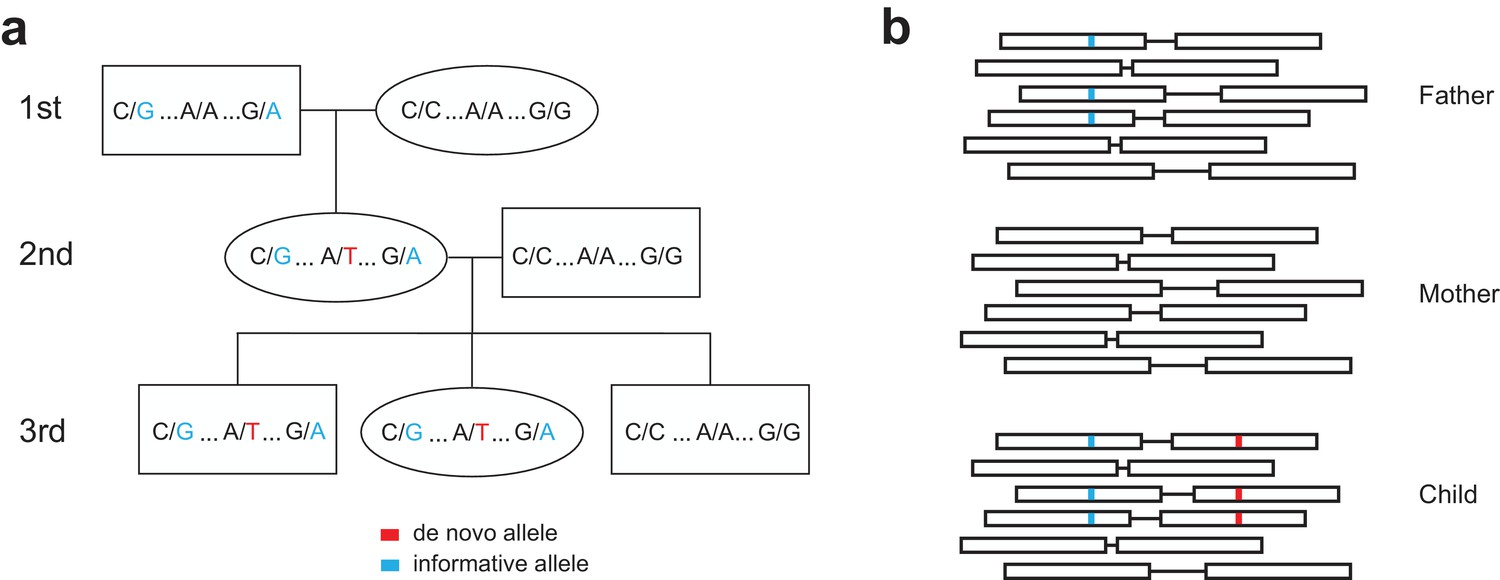
Estimating the rate of germline mutation using multigenerational CEPH/Utah pedigrees.
(a) The CEPH/Utah dataset comprises 33 three-generation families. Summaries of sequencing coverage for CEPH/Utah individuals are presented in Figure 1—figure supplement 1. After identifying candidate de novo mutations in the second generation (e.g., the de novo ‘T’ mutation shown in the second-generation father), it is possible to assess their validity both by their absence in the parental (first) generation and by transmission to one or more offspring in the third generation. (b) Total numbers of DNMs (both SNVs and indels) identified across second-generation CEPH/Utah individuals and stratified by parental gamete-of-origin. Boxes indicate the interquartile range (IQR), and whiskers indicate 1.5 times the IQR. Diagrams of phasing strategies for germline DNMs are presented in Figure 1—figure supplement 2.
Figure 1—figure supplement 1
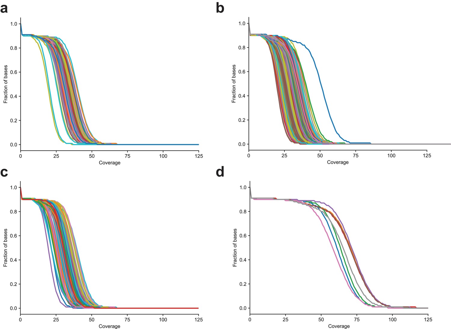
Distribution of sequencing coverage in CEPH/Utah samples (a) The fraction of bases greater than or equal to the specified coverage in the second generation, (b) third generation, (c) first-generation parents sequenced to 30X coverage, and (d) first-generation parents re-sequenced to 60X coverage.
https://doi.org/10.7554/eLife.46922.004
Figure 1—figure supplement 2
Determining the parent-of-origin for de novo mutations using transmission.
(a) We phased de novo mutations observed in the second generation by transmission to a third generation. We first searched ±200 kilobase pairs from the de novo allele (shown in red) for informative sites (shown in blue) present in one of the two first-generation parents of the second-generation individual. If the second-generation individual’s spouse does not possess these informative alleles, we can look in the children of the second-generation individual to see if they have inherited both the de novo allele and the nearby informative alleles. This pattern of inheritance is only possible if the de novo allele and informative alleles are on the same haplotype; thus, in this example, we see that the de novo allele is on the maternal grandfather’s haplotype, and is paternal in origin. (b) A toy sample of paired-end sequencing reads is shown for each member of a trio (mother, father, and child). In this strategy, we identify informative alleles (shown in blue) that are present in one of the two parents, and within a read length (500 bp) of the de novo allele in the child (shown in red). Then, we identify individual sequencing reads that span the de novo and informative alleles. If the de novo allele is always present in the same read as the informative allele, then we can phase the de novo allele to the parent with the informative allele, and vice versa.
Figure 2 with 2 supplements
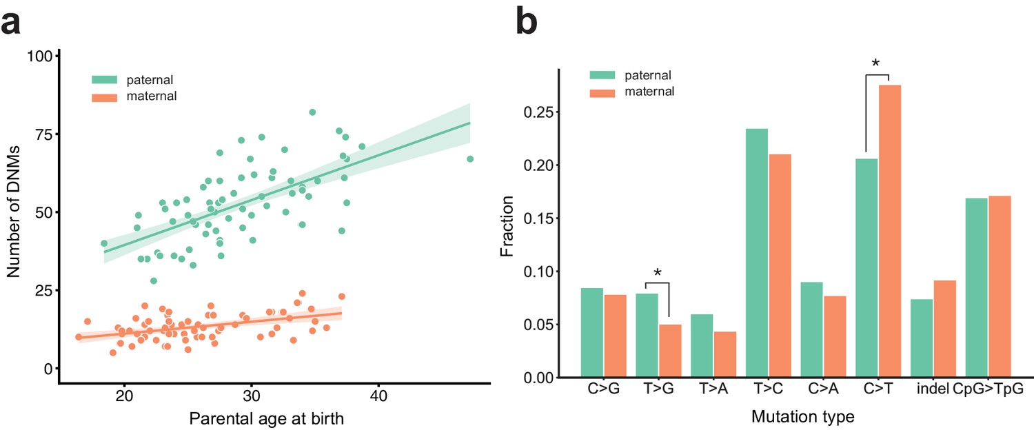
Effects of parental age and sex on autosomal DNM counts and mutation types in the second generation.
(a) Numbers of phased paternal and maternal de novo variants as a function of parental age at birth. Poisson regressions (with 95% confidence bands, calculated as 1.96 times the standard error) were fit for mothers and fathers separately using an identity link. Germline mutation rates, as a function of both paternal and maternal ages, are presented in Figure 2—figure supplement 1. (b) Mutation spectra in autosomal DNMs phased to the paternal (n = 3,584) and maternal (n = 880) haplotypes. Asterisks indicate significant differences between paternal and maternal fractions at a false-discovery rate of 0.05 (Benjamini-Hochberg procedure), using a Chi-squared test of independence. P-values for each comparison are: C > G: 0.719, T > G: 4.93e-3, T > A: 8.60e-2, T > C: 8.02e-2, C > A: 0.159, C > T: 7.65e-6, indel: 8.01e-2, CpG >TpG: 0.835. Mutation spectra stratified by parental ages are presented in Figure 2—figure supplement 2.
Figure 2—figure supplement 1
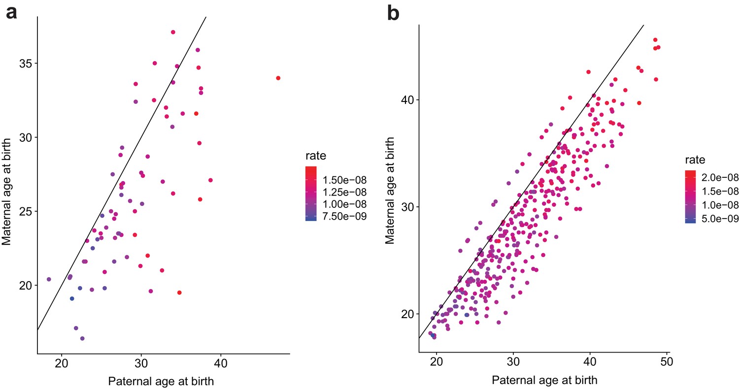
Contribution of maternal and paternal age to de novo mutation rates.
For (a) second- and (b) third-generation individuals in the CEPH/Utah cohort, plotted points show the relationship between paternal and maternal age at birth.Each point is colored by the autosomal SNV mutation rate in the individual; these rates were calculated by dividing the autosomal SNV DNM count in each child by that child’s autosomal callable fraction. Colors indicate the magnitude of the mutation rate (blue = lower, red = higher). Black lines indicate the trend for a 1:1 relationship between paternal and maternal age.
Figure 2—figure supplement 2
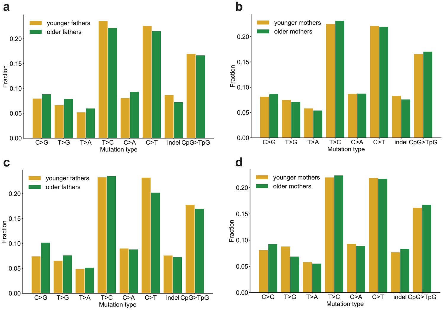
Comparison of mutation spectra in children born to older or younger parents.
Second-generation children were divided into two groups based on the ages of their parents at birth, and autosomal mutation spectra were compared between the two groups. In all panels, no significant differences were found at a false-discovery rate of 0.05 (Benjamini-Hochberg procedure), using a Chi-squared test of independence. (a) Comparison of DNMs in children born to fathers younger (n = 2,182) or older (n = 2,360) than the median paternal age of 29.2 years. P-values for each comparison are: C > G: 0.304, T > G: 0.140, T > A: 0.306, T > C: 0.248, C > A: 0.8.81e-2, C > T: 0.444, indel: 6.89e-2, CpG >TpG: 0.810. (b) Comparison of DNMs in children born to mothers younger (n = 2,225) or older (n = 2,317) than the median maternal age of 25.7 years. P-values for each comparison are: C > G: 0.580, T > G: 0.659, T > A: 0.554, T > C: 0.697, C > A: 0.918, C > T: 0.990, indel: 0.371, CpG >TpG: 0.678. (c) Comparison of DNMs in children born to fathers in the 25th percentile of youngest (n = 1,120) or oldest (n = 1,165) paternal ages (26.4 or 34 years). P-values for each comparison are: C > G: 1.73e-2, T > G: 0.428, T > A: 0.872, T > C: 0.979, C > A: 0.943, C > T: 7.77e-2, indel: 0.788, CpG >TpG: 0.706. (d) Comparison of DNMs in children born to mothers in the 25th percentile of youngest (n = 1,169) or oldest (n = 1,121) maternal ages (22.5 or 31.4 years). P-values for each comparison are: C > G: 0.327, T > G: 9.92e-2, T > A: 0.841, T > C: 0.975, C > A: 0.963, C > T: 0.940, indel: 0.598, CpG >TpG: 0.780.
Figure 3 with 2 supplements
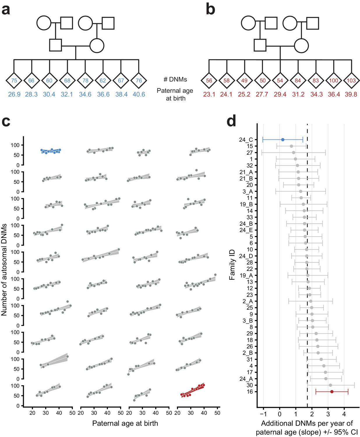
Parental age effects on autosomal germline mutation counts vary significantly among CEPH/Utah families.
Illustrations of pedigrees exhibiting the smallest (family 24_C, panel a) and largest (family 16, panel b) paternal age effects on third-generation DNM counts demonstrate the extremes of inter-family variability. Diamonds are used to anonymize the sex of each third-generation individual. The method used to separate CEPH/Utah pedigrees into unique groups of second-generation parents and third-generation children is presented in Figure 3—figure supplement 1. Third-generation individuals are arranged by birth order from left to right. The number of autosomal DNMs observed in each third-generation individual is shown within the diamonds, and the age of the father at the third-generation individual’s birth is shown below the diamond. The coloring for these two families is used to identify them in panels c and d. (c) The total number of autosomal DNMs is plotted versus paternal age at birth for third-generation individuals from all CEPH/Utah families. Regression lines and 95% confidence bands indicate the predicted number of DNMs as a function of paternal age using a Poisson regression (identity link). Families are sorted in order of increasing slope, and families with the least and greatest paternal age effects are highlighted in blue and red, respectively. (d) A Poisson regression (predicting autosomal DNMs as a function of paternal age) was fit to each family separately; the slope of each family’s regression is plotted, as well as the 95% confidence interval of the regression coefficient estimate. The same two families are highlighted as in (a). A dashed black line indicates the overall paternal age effect (estimated using all third-generation samples). Families are ordered from top to bottom in order of increasing slope, as in (c). A random sampling approach was used to assess the robustness of the per-family regressions to possible outliers; the results of these simulations are shown in Figure 3—figure supplement 2.
Figure 3—figure supplement 1
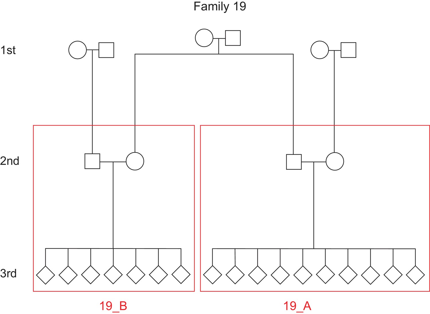
Defining unique families in the CEPH/Utah dataset.
The pedigree for a single family (family ID 19) is depicted. In this family, the third-generation individuals are first cousins and share a pair of grandparents. However, for the purposes of the inter-family variability presented in Figure 3, we defined ‘families’ as the unique groups of second-generation parents and their third-generation children. Thus, family ID 19 would be split into two unique families (19_A and 19_B), designated by the red boxes.
Figure 3—figure supplement 2
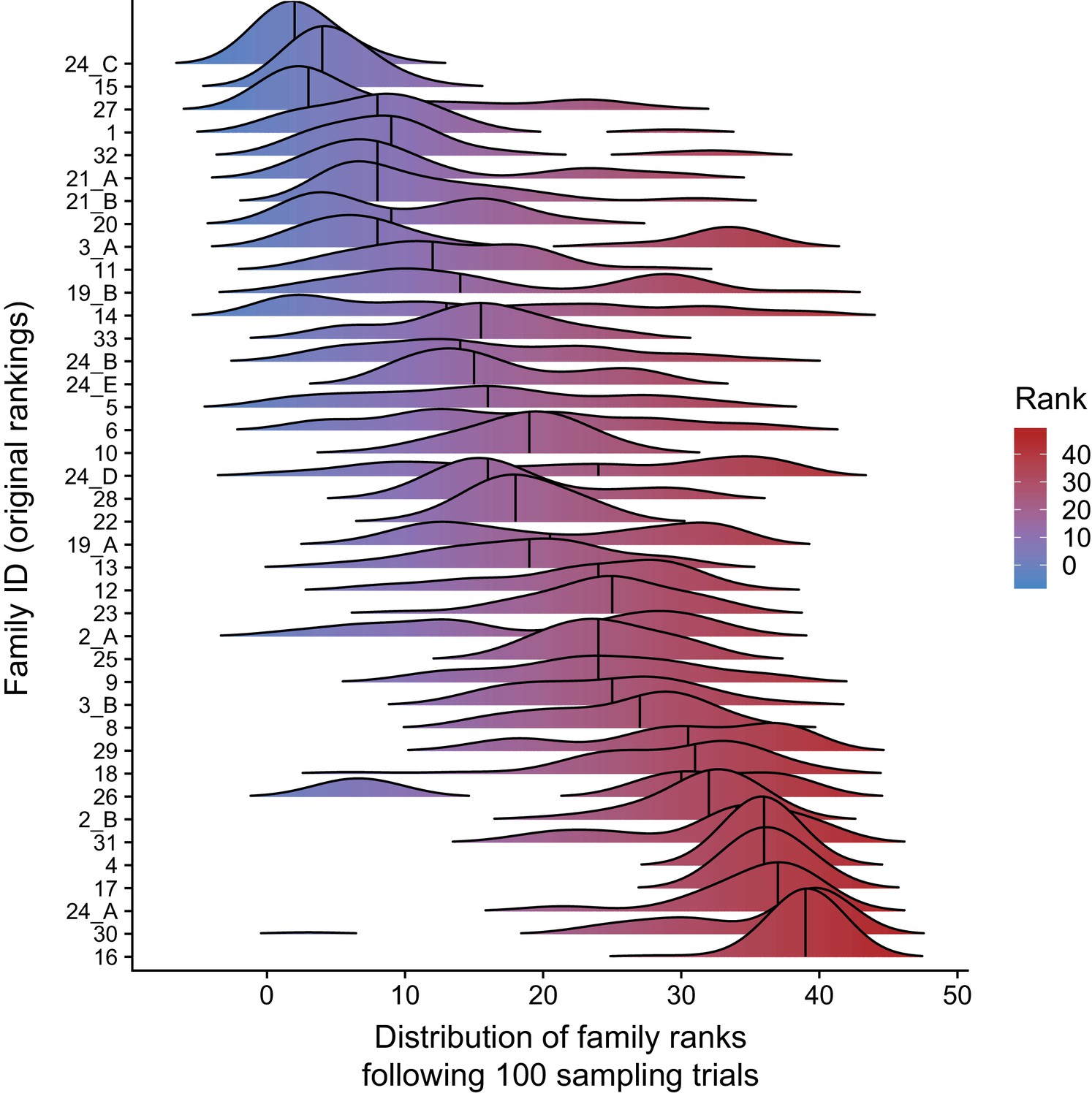
Paternal age effect ranks of CEPH/Utah families are robust to outlier samples.
For each CEPH/Utah family (i.e., unique set of second-generation and third-generation individuals), we randomly sampled 75% of the third-generation individuals in the family, fit a regression predicting autosomal DNM counts as a function of paternal age at birth, and calculated the ‘rank’ of that family’s paternal age effect (out of 40 total families). We then plotted the distribution of ranks across 100 trials for each family. Families’ density plots are ordered along the y-axis by the original ranks of each family (as determined using the full dataset, and originally shown in Figure 3d, where a rank of 1 corresponds to the smallest age effect, and a rank of 40 corresponds to the largest).
Figure 4
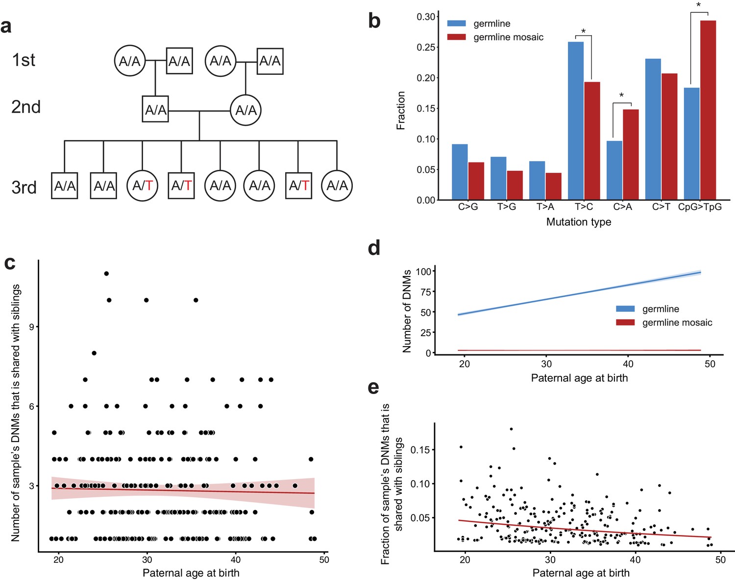
Identification of post-PGCS germline mosaicism in the second generation.
(a) Mosaic variants occurring during or after primordial germ cell specification (PGCS) were defined as DNMs present in multiple third-generation siblings, and absent from progenitors in the family. (b) Comparison of mutation spectra in autosomal single-nucleotide germline mosaic variants (red, n = 288) and germline de novo variants observed in the third generation (non-shared) (blue, n = 22,644). Asterisks indicate significant differences at a false-discovery rate of 0.05 (Benjamini-Hochberg procedure), using a Chi-squared test of independence. P-values for each comparison are: C > G: 6.84e-2, T > G: 0.169, T > A: 0.236, T > C: 1.51e-2, C > A: 4.31e-3, C > T: 0.385, CpG >TpG: 2.26e-6. (c) For each third-generation individual, we calculated the number of their DNMs that was shared with at least one sibling, and plotted this number against the individual’s paternal age at birth. The red line shows a Poisson regression (identity link) predicting the mosaic number as a function of paternal age at birth. (d) We fit a Poisson regression predicting the total number of germline single-nucleotide DNMs observed in the third-generation individuals as a function of paternal age at birth, and plotted the regression line (with 95% CI) in blue. In red, we plotted the line of best fit (with 95% CI) produced by the regression detailed in (c). (e) For each third-generation individual, we divided the number of their DNMs that occurred during or post-PGCS in a parent (i.e., that were shared with a sibling) by their total number of DNMs (germline +germline mosaic), and plotted this fraction of shared germline mosaic DNMs against their paternal age at birth.
Figure 5 with 1 supplement
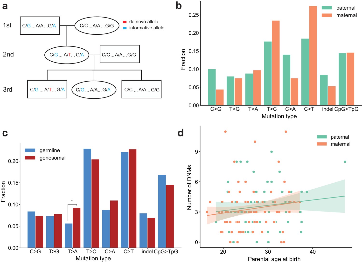
Identification of gonosomal mutations in the second generation.
(a) Gonosomal post-zygotic variants were identified as DNMs in a second-generation individual that were inherited by one or more third-generation individuals, but exhibited incomplete linkage to informative heterozygous sites nearby. (b) Comparison of mutation spectra in single-nucleotide gonosomal DNMs that occurred on the paternal (n = 249) or maternal (n = 226) haplotypes. No significant differences were found at a false-discovery rate of 0.05 (Benjamini-Hochberg procedure), using a Chi-squared test of independence. P-values for each comparison are: C > G: 3.05e-2, T > G: 0.972, T > A: 0.858, T > C: 0.148, C > A: 3.31e-2, C > T: 2.66e-2, indel: 0.247, CpG >TpG: 0.932. (c) Comparison of mutation spectra in autosomal single-nucleotide germline DNMs observed in the second-generation (non-gonosomal) (n = 4,542) and putative gonosomal mutations (n = 475) in the second generation. Asterisks indicate significant differences at a false-discovery rate of 0.05 (Benjamini-Hochberg procedure), using a Chi-squared test of independence. P-values for each comparison are: C > G: 0.517, T > G: 0.800, T > A: 2.32e-3, T > C: 0.255, C > A: 0.129, C > T: 0.805, indel: 0.446, CpG >TpG: 0.212. (d) Numbers of phased gonosomal variants as a function of parental age at birth. Poisson regressions (with 95% confidence bands) were fit for the mutations phased to the maternal and paternal haplotypes separately using an identity link. A diagram of an identification strategy for post-zygotic gonosomal DNMs (using only two generations) is presented in Figure 5—figure supplement 1.
Figure 5—figure supplement 1
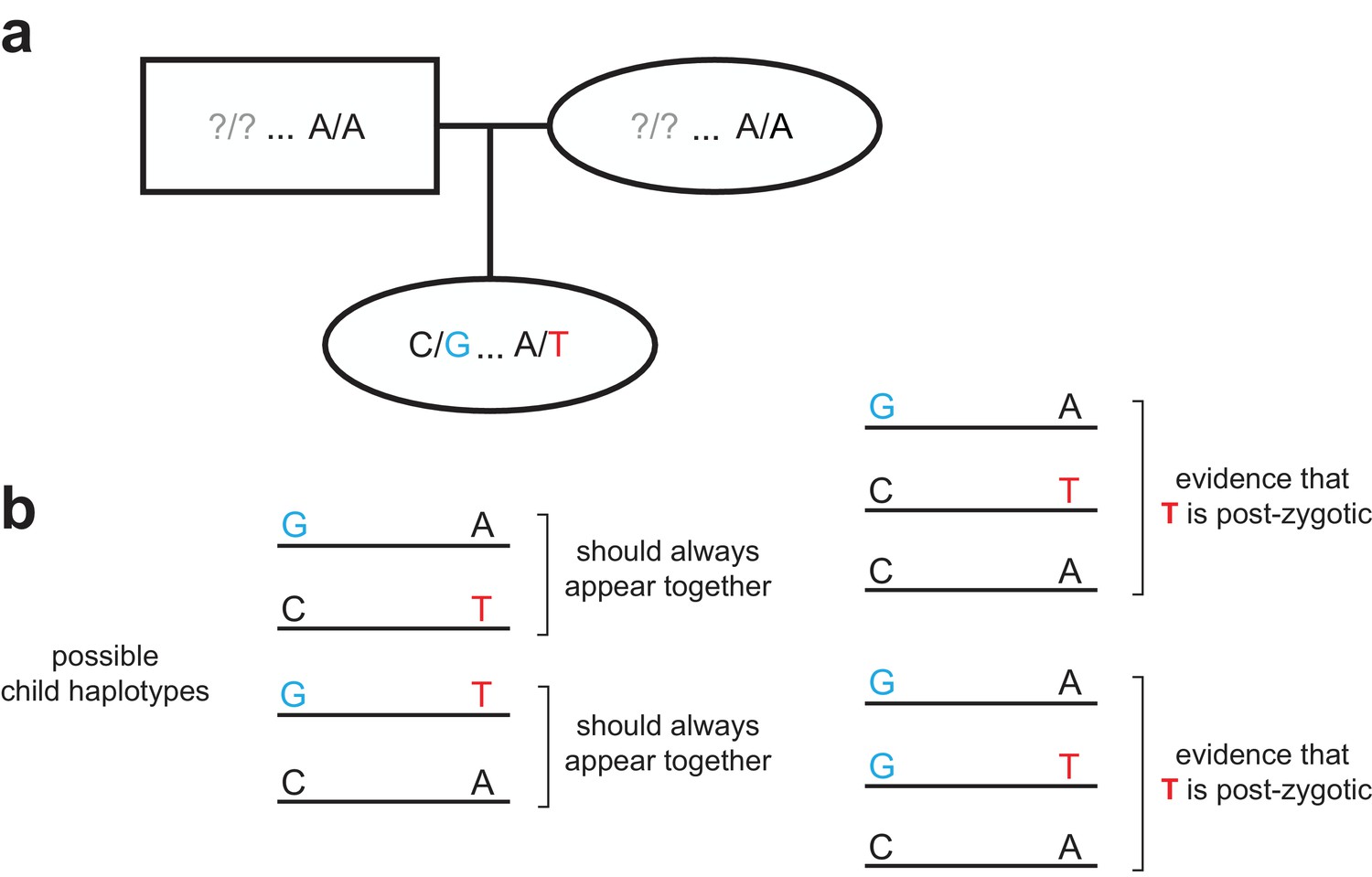
Strategy for identifying post-zygotic DNMs using two generations.
(a) Diagram of an example two-generation pedigree structure that is amenable to the post-zygotic detection strategy. In this example, the child has a de novo ‘T’ allele that is <= 500 bp downstream of a heterozygous ‘G’ allele. Question marks in the parents indicate that the child could have inherited the ‘G’ allele from either parent; unlike the read tracing strategy (Figure 1—figure supplement 2), a particular parent does not need to be ‘informative.’ (b) In the child’s reads, only two possible sets of linked haplotypes should be seen, assuming the de novo allele occurred in the germline of a parent. The presence of three distinct haplotypes, demonstrating incomplete linkage of the de novo and heterozygous alleles, indicates that the de novo ‘T’ allele is post-zygotic.
Author response image 1
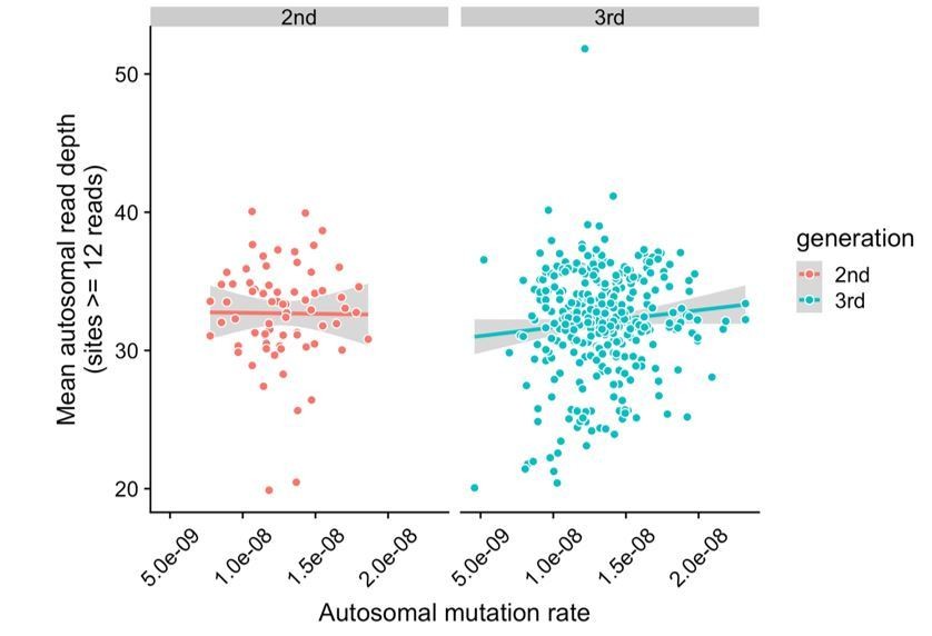
Lack of correlation between read depth and mutation rates in CEPH/Utah samples.
For each second- or third-generation CEPH/Utah sample, we calculated mean read depth across all autosomal base pairs covered by >=12 reads in all members of the trio. We then assessed whether there was a correlation between mean read depth and the autosomal mutation rate in these samples. For each generation, we fit a linear model predicting read depth as a function of autosomal mutation rate, and do not find a significant association in either generation at a p-value threshold of 0.05 (second-generation p = 0.92, third-generation p = 0.073).
Author response image 2
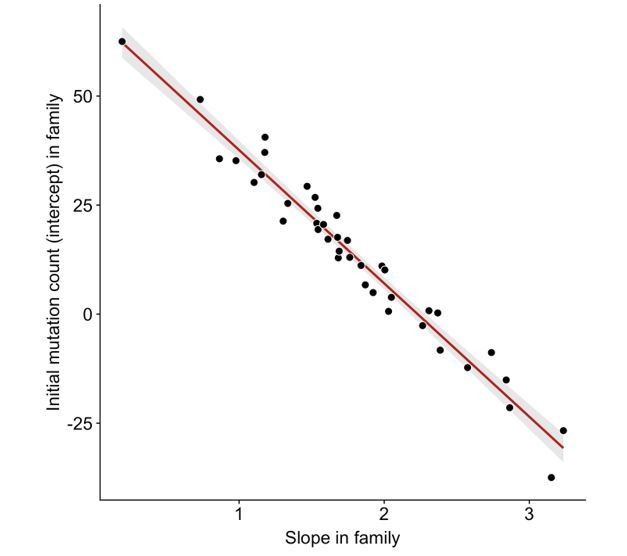
Anti-correlation between slope and intercept.
For each CEPH/Utah family, we fit a linear model predicting DNM counts as a function of paternal age (see Figure 3). We then assessed whether the slopes and intercepts of these regressions were correlated; overall, slope and intercept point estimates are negatively correlated in CEPH/Utah families (p < 2.2e-16).
Author response image 3
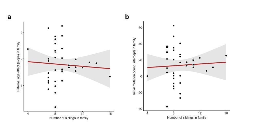
Lack of correlation between sibling number and either slope or intercept.
For each CEPH/Utah family, we fit a linear model predicting DNM counts as a function of paternal age (see Figure 3). We then assessed whether the number of third-generation siblings in these families was predictive of either the (a) slope or (b) intercept point estimate in the regression. Neither slope (p = 0.654) or intercept (p = 0.718) are significantly associated with sibling number.
Author response image 4

Allele balance distributions in transmitted and untransmitted DNMs.
Allele balance was calculated as the fraction of reads supporting the alternate (i.e., de novo) allele at a particular site. As there are substantially more transmitted than untransmitted DNMs in the plot, the y-axis is shown as the normalized count of DNMs.
Author response image 5
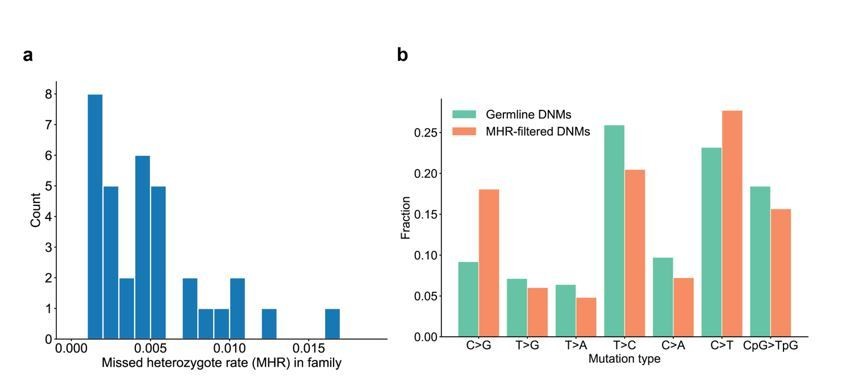
Range of missed heterozygote rates across CEPH families.
(a) For each unique set of second-generation parents and third-generation children, we counted the total number of DNMs in the third generation for which we saw evidence in the first generation (i.e., grandparents). The missed heterozygote rate (MHR) therefore represents the fraction of DNMs in each family that were likely “missed” in the second generation, as a percentage of the total number of DNMs identified in the third-generation children. (b) Comparison of mutation spectra in autosomal filtered germline third-generation DNMs (n=22,644) and autosomal third-generation DNMs that were removed due to evidence in a genotyped grandparent (n=83). No significant differences for particular mutation types were found at a false-discovery rate of 0.05 (Benjamini-Hochberg procedure) using a Chi-squared test of independence.
Tables
Key resources table
| Reagent type (species) or resource | Designation | Source or reference | Identifiers | Additional information |
|---|---|---|---|---|
| Software, algorithm | Genome Analysis Toolkit (GATK) | DePristo et al., 2011 | v3.5.0; RRID:SCR_001876 | |
| Software, algorithm | peddy | Pedersen and Quinlan, 2017a | v0.4.3; RRID: SCR_017287 | |
| Software, algorithm | cyvcf2 | Pedersen and Quinlan, 2017b | v0.11.2 | |
| Software, algorithm | mosdepth | Pedersen and Quinlan, 2018 | v0.2.4 | |
| Software, algorithm | pysam | https://github.com/pysam-developers/pysam | v0.15.2 | |
| Software, algorithm | python | https://www.python.org/ | v3.7.3; RRID:SCR_008394 | |
| Software, algorithm | R | https://www.r-project.org/ | v3.4.4; RRID:SCR_001905 | |
| Software, algorithm | Integrative Genomics Viewer (IGV) | Thorvaldsdóttir et al., 2013 | v2.4.11; RRID:SCR_011793 | |
| Software, algorithm | samtools | Li et al., 2009 | RRID: SCR_002105 | |
| Software, algorithm | BWA-MEM | Li, 2013 | v0.7.15; RRID:SCR_010910 |
Appendix 1—table 1
Results of ANOVA on fitted ‘family-aware’ model.
https://doi.org/10.7554/eLife.46922.022| Term (independent variable) | DoF | Deviance | Resid. DoF | Resid. Deviance | Pr(>Chi) |
|---|---|---|---|---|---|
| dad_age | 1 | 635.77 | 348 | 502.84 | < 2.2e-16 |
| family_id | 39 | 103.43 | 309 | 399.41 | 9.667e-9 |
| dad_age:family_id | 39 | 55.34 | 270 | 344.07 | 0.04328 |
Additional files
-
Supplementary file 1
Pedigree structures for all CEPH/Utah families.
All family and sample IDs have been anonymized, and the sexes of third-generation individuals have been hidden.
- https://doi.org/10.7554/eLife.46922.015
-
Supplementary file 2
IGV images of 100 randomly selected germline DNMs identified in the second generation.
In each image, the first two tracks contain alignments from the first-generation parents, and the third track contains the alignments for the second-generation child. Reads with mapping quality <20 are not included, as they were not considered by our variant calling pipeline, and mismatched bases are shaded by quality score (more transparent = lower base quality).
- https://doi.org/10.7554/eLife.46922.016
-
Supplementary file 3
IGV images of 100 randomly selected germline.
DNMs identified in the third generation In each image, the first two tracks contain alignments from the second-generation parents, and the third track contains the alignments for the third-generation child. Reads with mapping quality <20 are filtered out, as they were not considered by our variant calling pipeline, and mismatched bases are shaded by quality score (more transparent = lower base quality).
- https://doi.org/10.7554/eLife.46922.017
-
Supplementary file 4
IGV images of all putative post-PGCS mosaic mutations In each image, the first two tracks contain alignments from the two second-generation parents in the pedigree.
All tracks below contain alignments from the third-generation children that share a DNM at the site. Reads with mapping quality <20 are filtered out, as they were not considered by our variant calling pipeline, and mismatched bases are shaded by quality score (more transparent = lower base quality).
- https://doi.org/10.7554/eLife.46922.018
-
Supplementary file 5
IGV images of all putative gonosomal mutations identified in the second generation.
In each image, the first two, three, or four tracks contain alignments from the grandparents in the pedigree (i.e., paternal grandmother and grandfather, maternal grandmother and grandfather). In some families, one or two of the first-generation grandparents were not sequenced (see Supplementary file 1). The two tracks below contain alignments from the second-generation individual with the putative gonosomal mutation and that second-generation individual’s spouse. The remaining tracks below contain alignments from the third-generation individuals that inherited the gonosomal mutation. Reads with mapping quality <20 are filtered out, as they were not considered by our variant calling pipeline, and mismatched bases are shaded by quality score (more transparent = lower base quality).
- https://doi.org/10.7554/eLife.46922.019
-
Transparent reporting form
- https://doi.org/10.7554/eLife.46922.020
Download links
A two-part list of links to download the article, or parts of the article, in various formats.
Downloads (link to download the article as PDF)
Open citations (links to open the citations from this article in various online reference manager services)
Cite this article (links to download the citations from this article in formats compatible with various reference manager tools)
Large, three-generation human families reveal post-zygotic mosaicism and variability in germline mutation accumulation
eLife 8:e46922.
https://doi.org/10.7554/eLife.46922


