Functional clustering of dendritic activity during decision-making
- Janelia Research Campus, Howard Hughes Medical Institute, United States
Figures
Figure 1 with 3 supplements
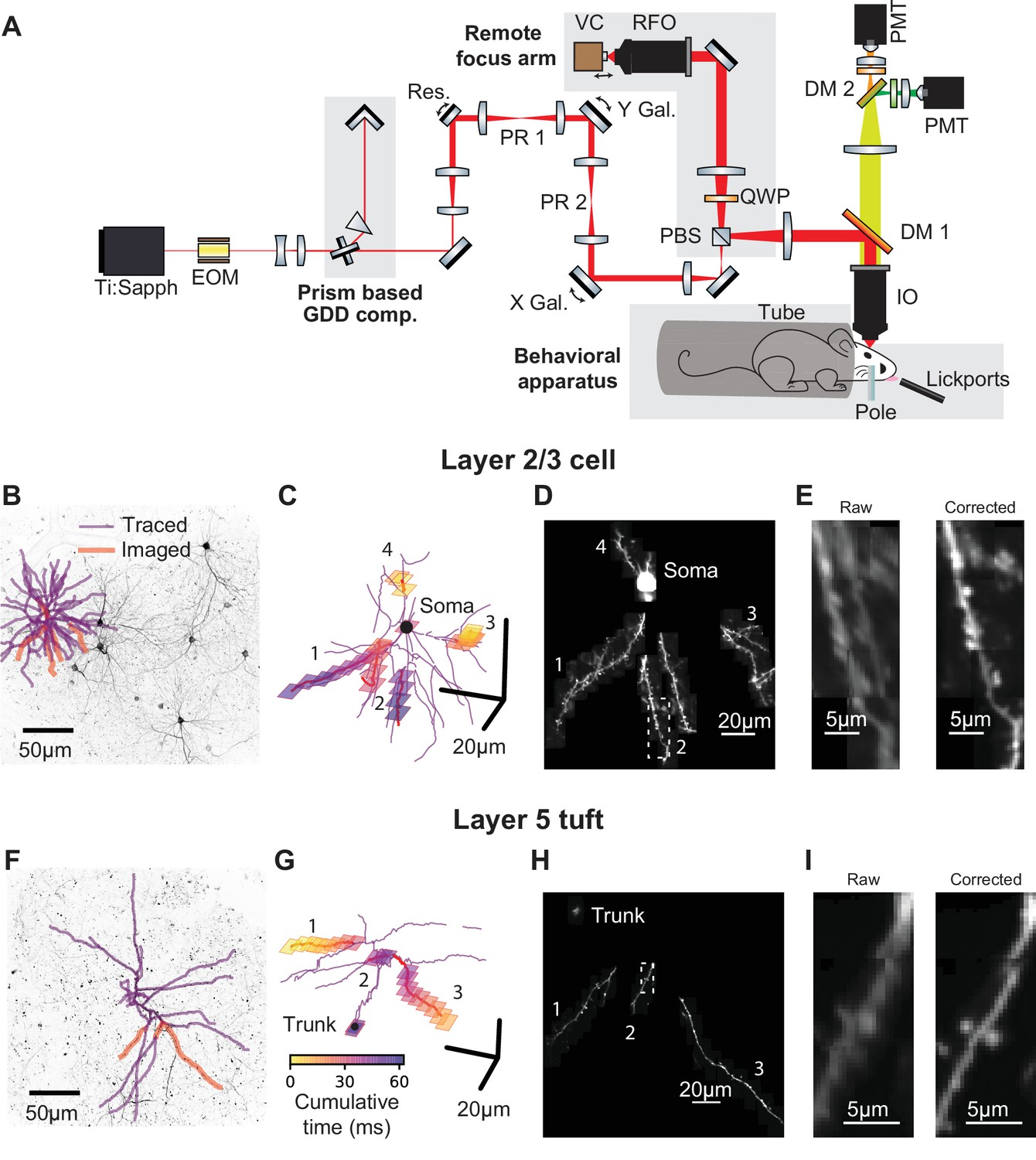
Targeted high-speed imaging in behaving mice.
(A) Optical layout for high-speed, high-resolution imaging in three dimensions. An x-axis mirror galvanometer, remote focusing arm, and prism-based GDD compensation unit were added to a high resolution (NA = 1.0) resonant two photon microscope. EOM, electro-optic modulator; GDD, group delay dispersion; Res., 8 kHz resonant scanner; PR, pupil relay; Gal., galvanometer; PBS, polarizing beam splitter; QWP, quarter wave plate; RFO, remote focusing objective; VC, voice coil; DM, dichroic mirror; IO, imaging objective; PMT, photomultiplier tube. (B) Maximum intensity projections (MIP) of anatomical stack collected from Syt17-Cre x Ai93 (pia to 306 um depth) mice. Traced dendrite (purple lines) and example targets (red lines) for an example imaging session. (C) Spatial and temporal distribution of the frames that compose the example functional imaging sequences in (B). (D) Average MIP of 30 min of the functional imaging sequence shown in (B, C). (E) Close-up of the dendritic branch outlined in (D) before and after motion correction. (F–I) same as (B–E) for a layer 5 cell (MIP in (F) is pia to 560 um depth). See also Figure 1—figure supplement 1 for characterization of the transgenic lines and Figure 1—figure supplement 2 for details on motion registration.
Figure 1—figure supplement 1
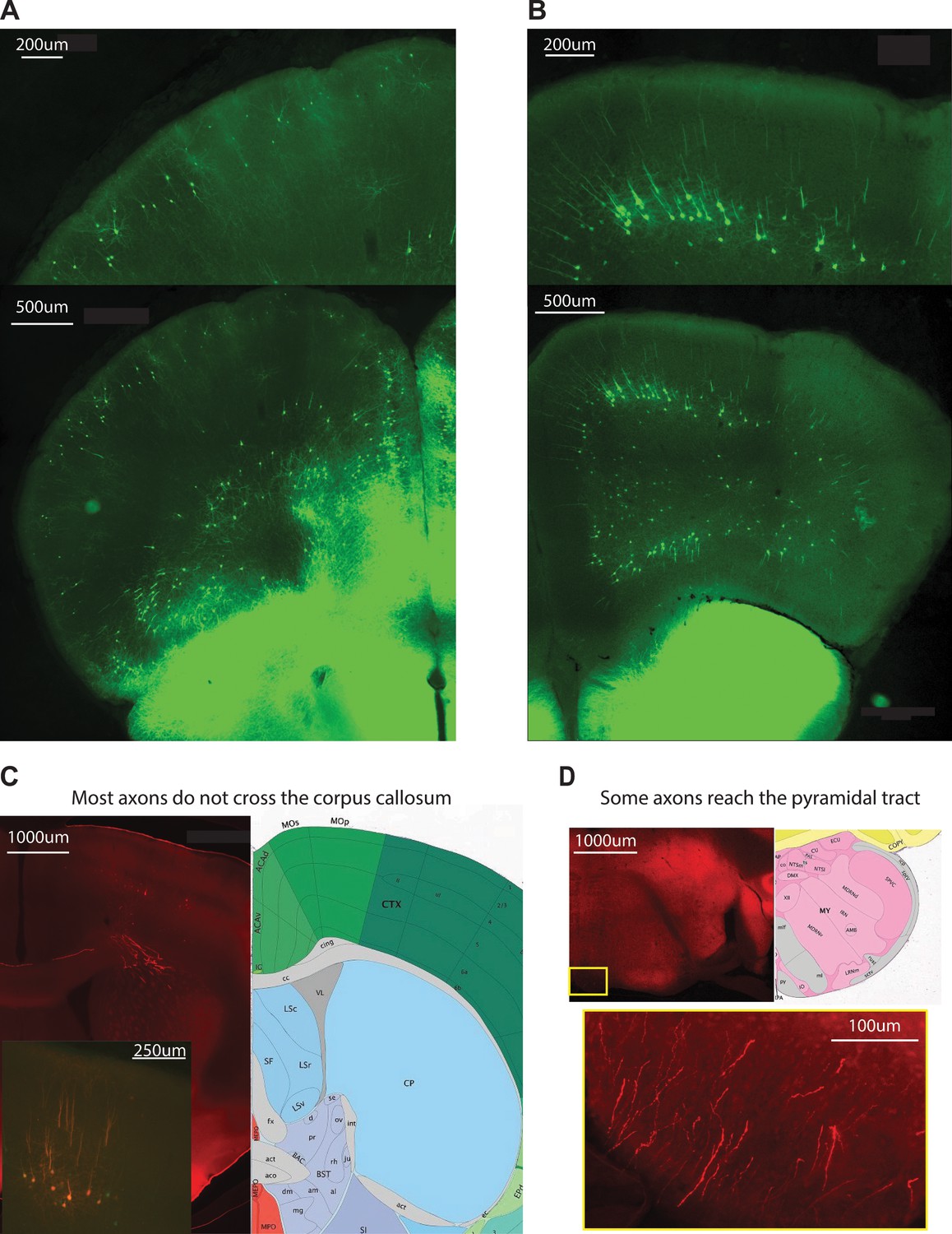
Histological characterization of transgenic mouse lines.
(A) GCaMP labeling in an example coronal section of Syt17-Cre x Ai93 approximately 1.5 mm anterior to bregma. (B) GCaMP labeling in an example coronal section of OE25-Cre x Ai93 approximately 1.5 mm anterior to bregma. (C) CRE dependent tdTomato injection to a OE25-Cre x Ai93 mouse to enable to trace axons of L5 ALM neurons. Most axons do not cross the midline. Inset, the injection site. (D) Some axons are seen in the pyramidal tract.
Figure 1—figure supplement 2
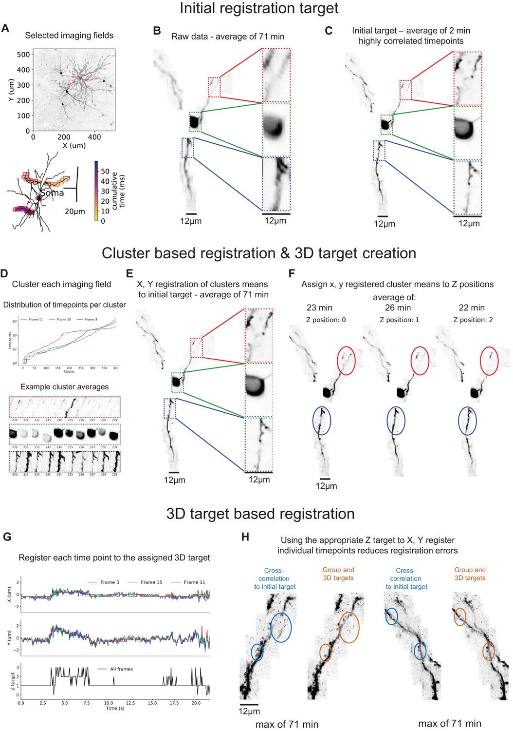
Image regestration example.
(A) Tracing of dendrites (top) and spatiotemporal distribution of imaging frames (bottom) for an example L2/3 cell imaging session. (B) Maximum intensity projection (MIP, 80 μm z-axis) of the average of 71 min of continuous imaging before motion correction. Zoom-in images from three example frames (colored boxes) show that individual dendritic spines are difficult to discern because of motion averaging. (C) MIP based on the average a highly correlated subset of samples, determined using k-means clustering (same session as in B). This average volume is used as an initial target for registration. (D) Samples of each frame across time were divided into 400 clusters by k-means. Samples within each cluster were then averaged to increase the signal-to-noise ratio. (E) MIP after lateral shifts were applied to all samples within each frame cluster based on registration of the corresponding frame cluster average (D) to the initial target (C) via cross-correlation. (F) MIPs of the average of samples from 3 estimated 3D targets identified by clustering, ordering, and grouping of the laterally registered data (E, see Materials and methods for details). At the end of this process, every sample and frame is independently assigned to one of 4–8 3D target volumes. (G) Estimated shifts from sample-by-sample constrained registration of each frame to assigned 3D targets. (H) MIPs along the z-axis and time for two dendritic branches comparing the results of cross-correlation-based registration of frames to the initial target (blue) versus constrained registration to assigned z-shifted targets (brown). Note ‘doubling’ (left example branch, blue circles) from systematic registration errors and blurring (right example branch, blue circles) using standard cross-correlation that is not present with constrained registration to assigned 3D targets (brown circles).
Figure 1—video 1
Registration Example.
Top, target for registration is in yellow, single timepoints are in blue. Red arrows indicate the calculated shifts per imaging field. Arrows are 3x real size to emphasize the pixel sized shifts. Bottom, traces of the activity of the soma (blue) and detected licks (green stars).
Figure 2 with 3 supplements

Dendrite and spine calcium activity.
(A) Mice were trained to lick either a right or left target based on pole location. The pole was within reach of the whiskers during the sample epoch. Mice were trained to withhold licks until after a delay and auditory response cue. (B) Top, example somatic (black), dendritic (magenta), and spine (green) calcium signals from a layer 2/3 example session (as shown Figure 1B–E). Bottom, maximum intensity projections (au) and branch insets at selected times (dashed vertical lines in upper traces). Note independent spine activity at time i. (C) Same as (B) but for the layer five example session (as in Figure 1F–I). The apical trunk (black) was targeted as a reference for global activity. Note branch-specific sustained activity at time ii.
Figure 2—figure supplement 1
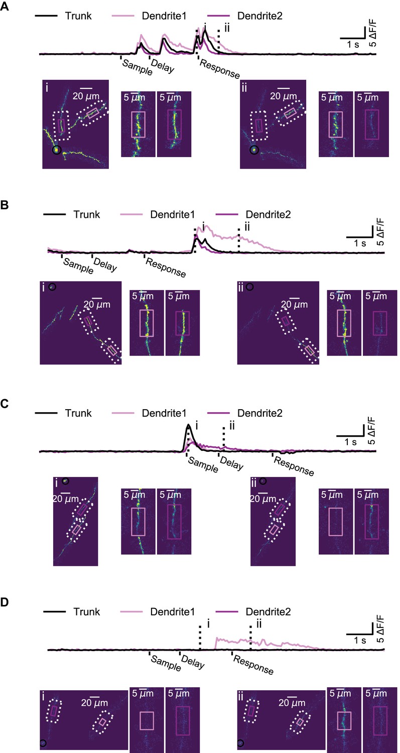
Examples of branch-specific persistent calcium activity.
(A) Example of branch-specific persistence of calcium activity following multi-branch events in the dendrites of a L2/3 neuron (soma not imaged in this session). Top, example apical trunk (black) and two dendritic branches (light and dark magenta) calcium signals. Bottom, maximum intensity projections (au) and branch insets at example times (dashed vertical lines in upper traces). Note persistent activity in one dendritic branch (light magenta) that is not present in the other (dark magenta). (B) Same as (A), but for the apical tuft of a L5 neuron. (C) Another example of (B). (D) Example of a putative independent branch event in the apical tuft of a L5 neuron. Note the large increase in calcium signal in one branch (light magenta), but no detectable increase in the apical trunk or other branch.
Figure 2—video 1
Layer 2/3 Example Calcium Activity.
Top, post-registration activity (AU) for the soma (white), an example spine (green circle), and a segment of dendrite (magenta arrow). Bottom, ΔF/F of the soma (white), spine (green), and dendrite (magenta). This is the same segment of activity as in Figure 2B.
Figure 2—video 2
Layer 5 Example Calcium Activity.
Top, post-registration activity (AU) for the trunk (white), an example spine (green circle), and a segment of dendrite (magenta arrow). Bottom, ΔF/F of the soma (white), spine (green), and dendrite (magenta). This is the same segment of activity as in Figure 2C.
Figure 3 with 2 supplements
Coincidence of dendritic calcium transients with events in the soma and apical trunk.
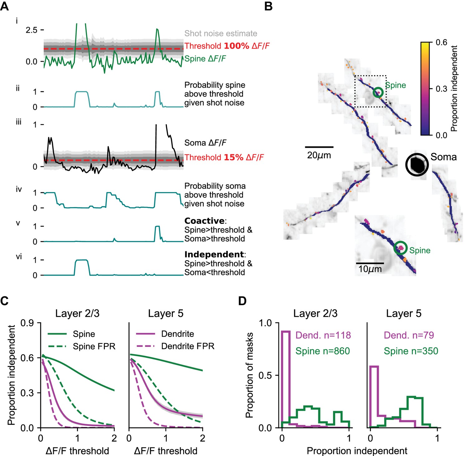
(A) Estimation of isolated spine activity as a function of threshold. (i) Example spine ΔF/F (green), threshold (red - 100% ∆F/F) and estimated uncertainty in ΔF/F due to shot-noise (gray shading). (ii) Probabilities of the spine to be above threshold. (iii, iv) same as (i, ii), but for the soma (black) with a lower threshold (15% ∆F/F). (v) Probability of co-activity. (vi) Probability of independent activity. (B) The proportion of independent activity in spines and dendrites with soma used as reference, example session. (C) Proportion independent as a function of threshold averaged across all spines (green) and dendrites (magenta). Left, L2/3 basal and apical dendrites with soma used as reference. Right, L5 tuft dendrites with apical trunk used as reference. Shaded region: SEM. Dotted lines: estimated false positive rate (FPR). (D) Distribution of the mean proportion independent activity of spines (green) and dendrites (magenta) of layer 2/3 cells (left) and L5 tuft (right). Note, L5 dendrites have a more rightward skewed distribution. See Figure S3 for the full distributions of co-active, independent and false positive rate as a function of thresholds. Layer 2/3: N = 6 mice; 13 neurons. Layer 5: N = 4 mice; five neurons.
Figure 3—figure supplement 1
Coincidence activity analysis with different thresholds.
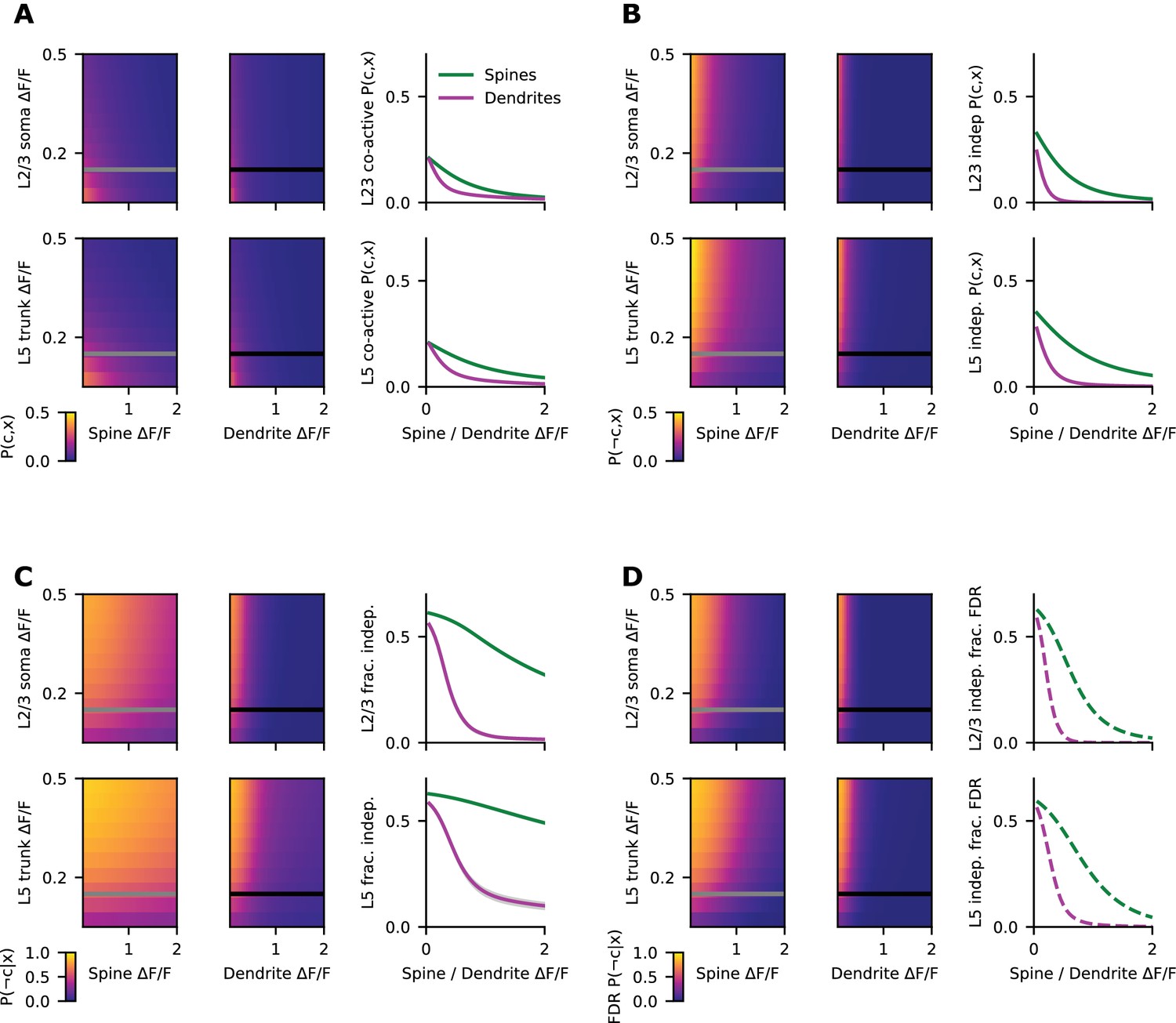
(A) Proportion of time that dendritic spines (left heatmaps) or dendritic segments (right heatmaps) are co-active with the bAP reference signal (soma or apical trunk) as a function of arbitrary threshold and estimated shot-noise. Rightmost plots show the fraction of time co-active as a function of ΔF/F threshold on spine (green) or dendritic segment (magenta) with reference threshold fixed at 15% ΔF/F (dashed white line in heatmaps). (B) Same as (A), but for the proportion of time that spines or dendritic segments are above threshold and the reference signal is below threshold. (C) Same as (B), but for the fraction of time that the reference signal is not above threshold, given that spines or dendritic segments are above threshold (‘fraction independent’). (D) Estimated false positive rate (FPR) for the faction independent shown in (C).
Figure 3—figure supplement 2
Excluding independent activity before or after reference activity.
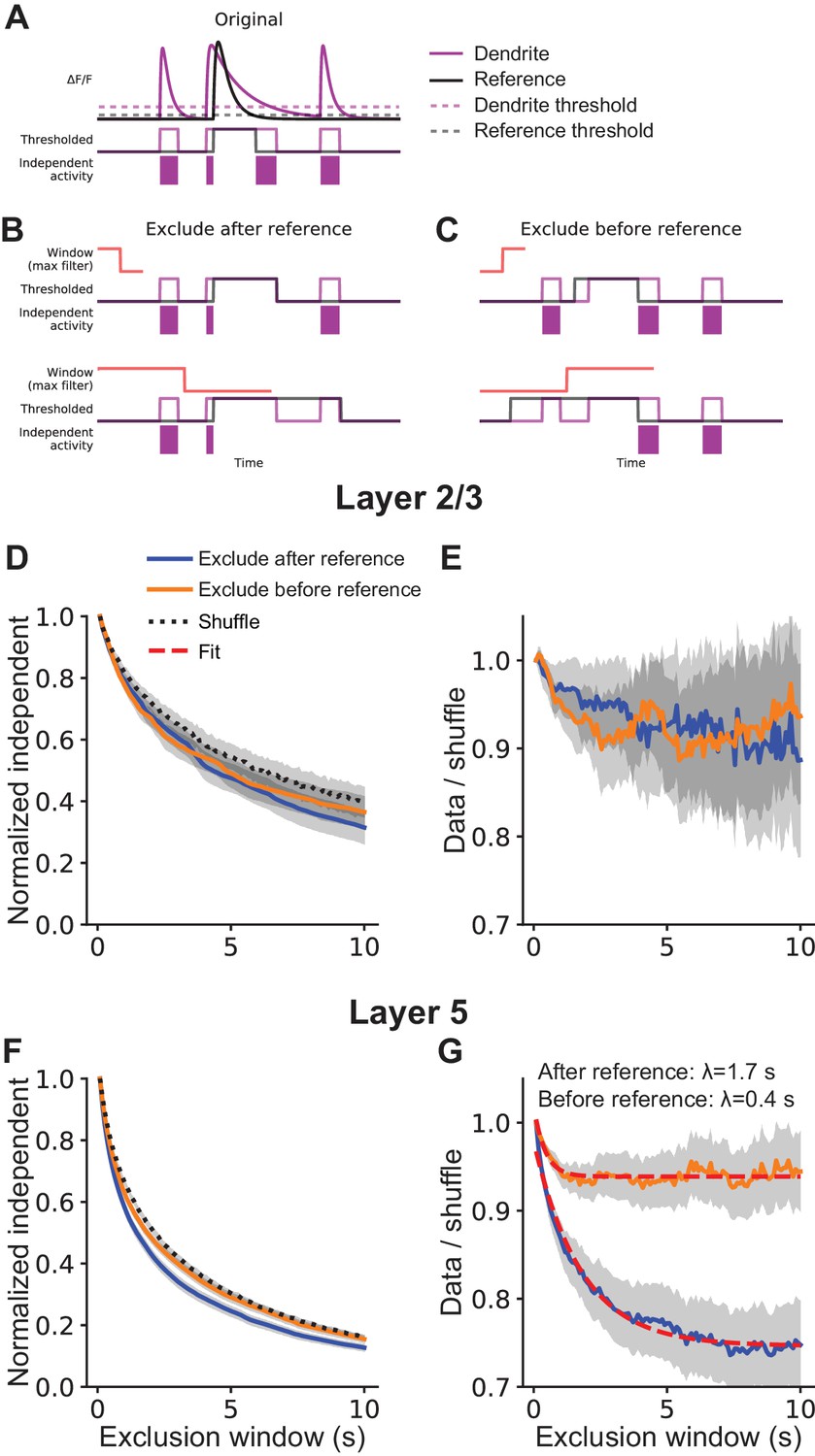
(A) Illustration of the transformation of reference (black) and dendritic (magenta) fluorescence signals to an estimate of independent activity (see Figure 3A; Materials and methods). (B) To exclude independent activity after reference activity, the thresholded reference signal is processed with a maximum filter (‘exclusion window’) that extends the thresholded reference signal forward in time. (C) Same as (B), but excluding independent activity before reference activity. (D) Decline of proportion independent activity in 30 μm segments of the dendrites of layer 2/3 neurons as the exclusion window (see Materials and methods) is extended before (orange line) or after (blue line) the reference signal. Dotted line is shuffle of the reference signal. Normalized independent is the proportion independent normalized by the value at no additional exclusion. Only dendrite segments with proportion independent above 0.05 were included (N = 17 segments). (E) Ratio of normalized independent and shuffle values in (D) as the exclusion window is increased. (F) Same as (D), but for the tuft dendrite of layer five neurons (N = 43 segments). (G) Same as (E), but for the tuft dendrite of layer five neurons. Red dashed lines are single-exponential fits to the data and λ is the time constant of each fit.
Figure 4 with 2 supplements
Local selectivity after removing the bAP component.
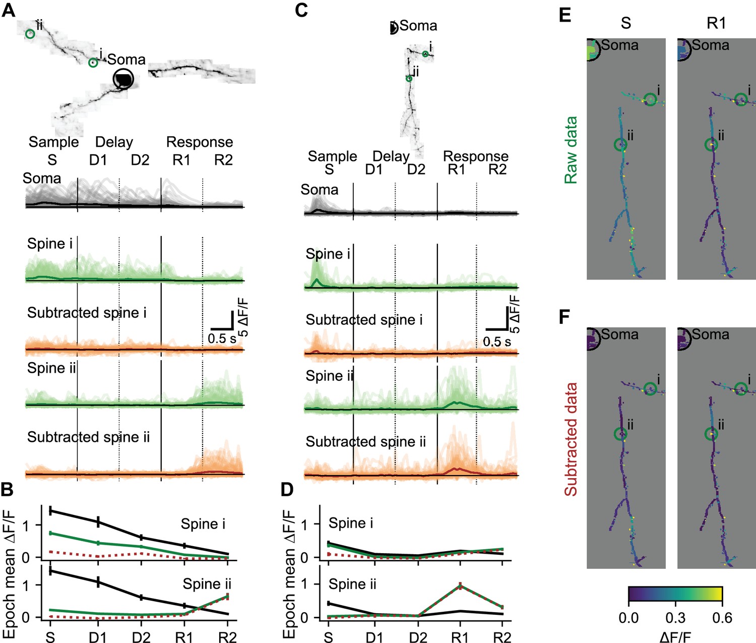
(A) Subtraction of the bAP component from spine signals and estimation of trial average responses for two example spines. Image: MIP of an example L2/3 cell. Light lines: ΔF/F for all 110 correct right trials. Dark lines: trial-average ΔF/F. Black: Soma. Green: Spine before bAP subtraction. Brown: Spine after bAP subtraction. (B) Mean and standard error by trial epoch across all correct right trials of the spines in (A) with the same color-code. Note that most of the activity is being subtracted in spine i, but independent activity is not being subtracted in the response epoch of spine ii. (C, D) Same as (A, B) for a different L2/3 cell. (E) Trial-average responses of right sensory (S) and early response (R1) epochs for all dendrite segments and spines in the session shown in (C). (F) Same as (E) after removal of the estimated bAP component. See also Figure 4—figure supplement 1 for an example subtraction of two spines.
Figure 4—figure supplement 1
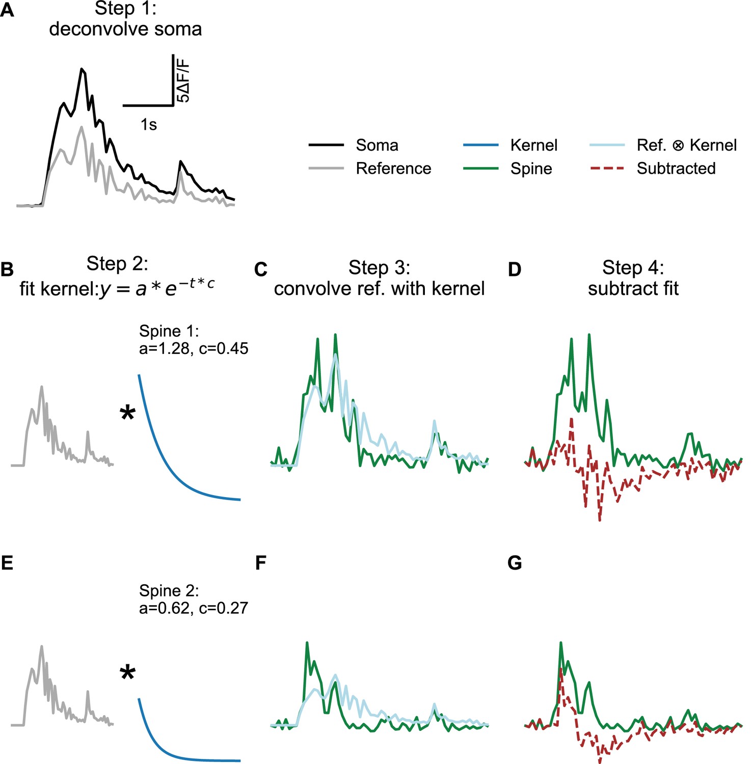
Process for removing the estimated bAP-component of spine and dendritic segment signals.
(A) Example reference signal (soma; black line). The reference signal was deconvolved by FOOPSI (Pnevmatikakis et al., 2016; Vogelstein et al., 2010) with parameters set to bias towards a dense reconstruction (gray line, see Materials and methods). (B–D) Subtraction for an example spine signal. For each spine or segment, we found an exponential kernel (B) that when convolved with the reference signal (C) minimized the sum of squared residuals between the convolved reference signal and the spine or segment (D). Note that this spine has very little residual activity after bAP-component removal. (E–G) Same as B-D, but for a different spine recorded simultaneously from the same cell. Note that this spine was fit to a kernel with about half the amplitude and decay as the spine in (B). Also, note the substantial residual activity after bAP-component removal.
Figure 4—figure supplement 2
Example of independent and trial averaged activity in a L5 tuft dendrite segment.
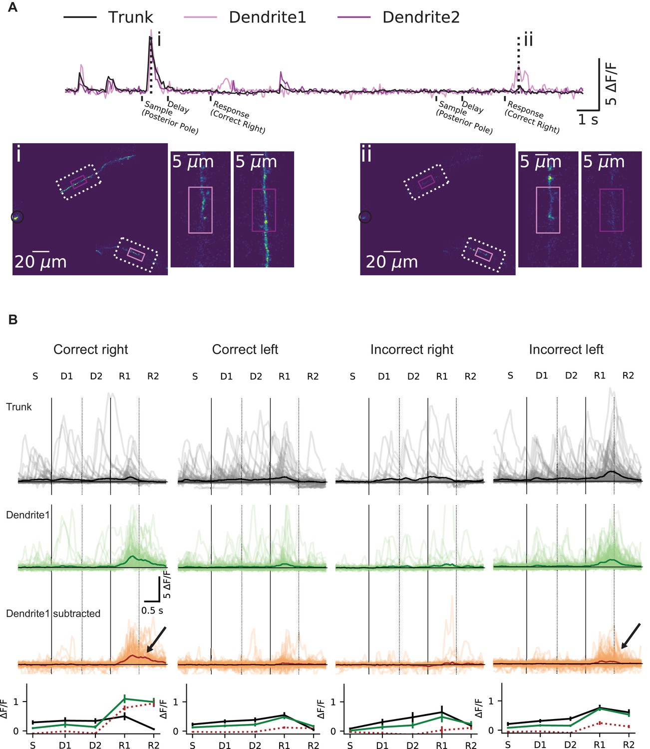
(A) Top, example apical trunk (black) and two dendritic branches (light and dark magenta) calcium signals. Bottom, maximum intensity projections (au) and branch insets at example times (dashed vertical lines in upper traces). Note coincident activity in time point (i) compared to independent activity at time point (ii) following the go cue (response epoch). (B) Trial-aligned activity of the trunk (black) and dendrite1 shown in (A) for both correct and incorrect trials. Note strong selectivity in the dendrite segment for trials in which the mouse licks to the right (i.e., correct right and incorrect left trials – see arrows) that was not present in the trunk.
Figure 5 with 1 supplement
Dendrite and spine calcium signals exhibit diverse selectivity for trial epoch and trial type.
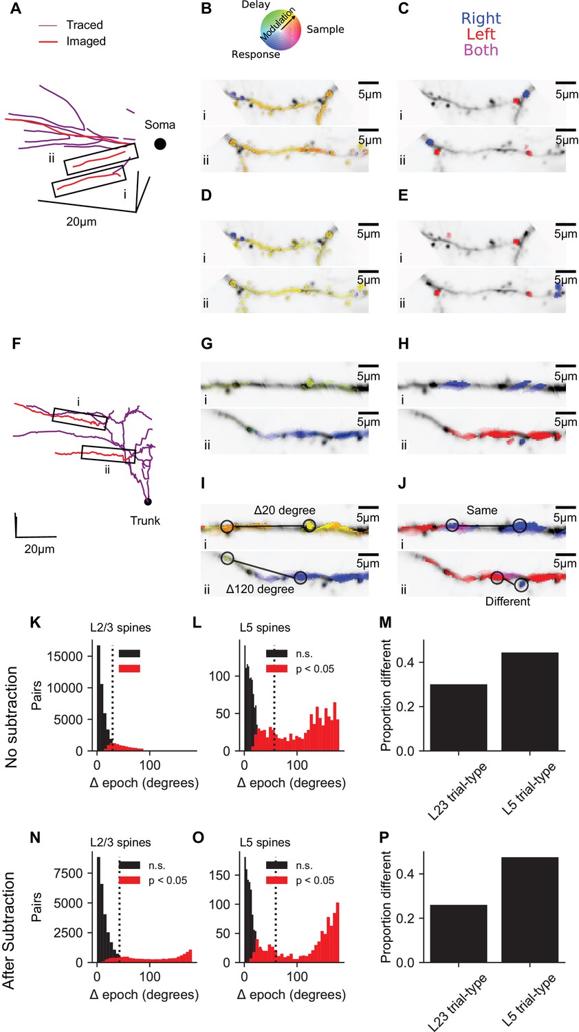
(A) Location of simultaneously imaged dendrite (red lines) relative to the soma (black dot) and connecting dendrite (purple) that was not imaged for an example imaging session of a L2/3 cell. (B) Epoch selectivity for masks at two locations denoted by black boxes in (A). Mean sample, delay, and response epoch ΔF/F provided the magnitude for three vectors separated by 120°. The angle of the vector average in a polar RGB space determined the color of each mask. Only masks with significant epoch selectivity (nonparametric ANOVA, p<0.01 and epoch angle SE <30 degrees, see Materials and methods) are colored. (C) same as (B) but for trial-type selectivity. Masks significantly selective (permutation t-test, p<0.05 with Bonferroni correction) for right are blue, selective for left are red, and selective for both right and left depending on epoch are purple. (D, E) Same as (B, C), but with bAP subtraction. (F–J) Same as (A–E), but for an example L5 tuft session. Black dot in (F) denotes apical truck. (K) Distribution for L2/3 neurons of differences in epoch selectivity between epoch selective spines (epoch angle CI <30 degrees) on the same neuron for L2/3 neurons (N = 56568 pairs, 2038 spines). Red: Significantly different (p<0.05; bootstrap test on epoch angle). Black: Not significantly different. Dotted line: Mean angle across all pairs. (L) Same as (K), but for L5 tuft (N = 2060 pairs, 237 spines). (M) Of trial-type selective spines, proportion of spine pairs with different trial-type selectivity (L2/3: N = 16485 pairs, 905 spines; L5: N = 788 pairs, 135 spines). (N–P) Same as (K–M), but with bAP subtraction (N: N = 38677 pairs, 1692 spines; O: N = 1958 pairs, 235 spines; P,L2/3: 15284 pairs, 802 spines; P,L5: 7328 pairs, 143 spines).
Figure 5—figure supplement 1
Dendrite Signals Exhibit Diverse Selectivity for Trial Epoch and Trial Type.
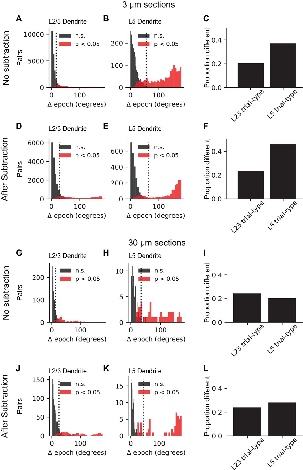
(A) Distribution for L2/3 neurons of differences in epoch selectivity between epoch selective dendrite segments of 3 um (epoch angle CI <30 degrees) on the same neuron for L2/3 neurons (N = 28389 pairs, 1431 segments). Red: Significantly different (p<0.05; bootstrap test on epoch angle). Black: Not significantly different. Dotted line: Mean angle across all pairs. (B) Same as (A), but for L5 tuft (N = 3209 pairs, 290 segments). (C) Of trial-type selective dendrite segments, proportion of dendrite pairs with different trial-type selectivity (L2/3: N = 14197 pairs, 814 segments; L5: N = 2038 pairs, 229 segments). (D–F) Same as (A–C), but with bAP subtraction (D: N = 21892 pairs, 1303 segments; E: N = 4061 pairs, 327 segments; F,L2/3: 9428 pairs, 684 segments; F,L5: 2216 pairs, 217 segments). (G–L) Same as (A–F), but with 30 um dendrite sections (G: N = 1090 pairs, 292 segments; H: N = 141 pairs, 61 segments; I,L2/3: 638 pairs, 192 segments; I,L5: 137 pairs, 60 segments; J: N = 968 pairs, 294 segments; K: N = 160 pairs, 71 segments; L,L2/3: 510 pairs, 165 segments; L,L5: 153 pairs, 59 segments).
Figure 6 with 2 supplements
Interpretation of dendritic calcium signals before and after removal of the estimated contribution from back-propagating action potentials (bAPs).
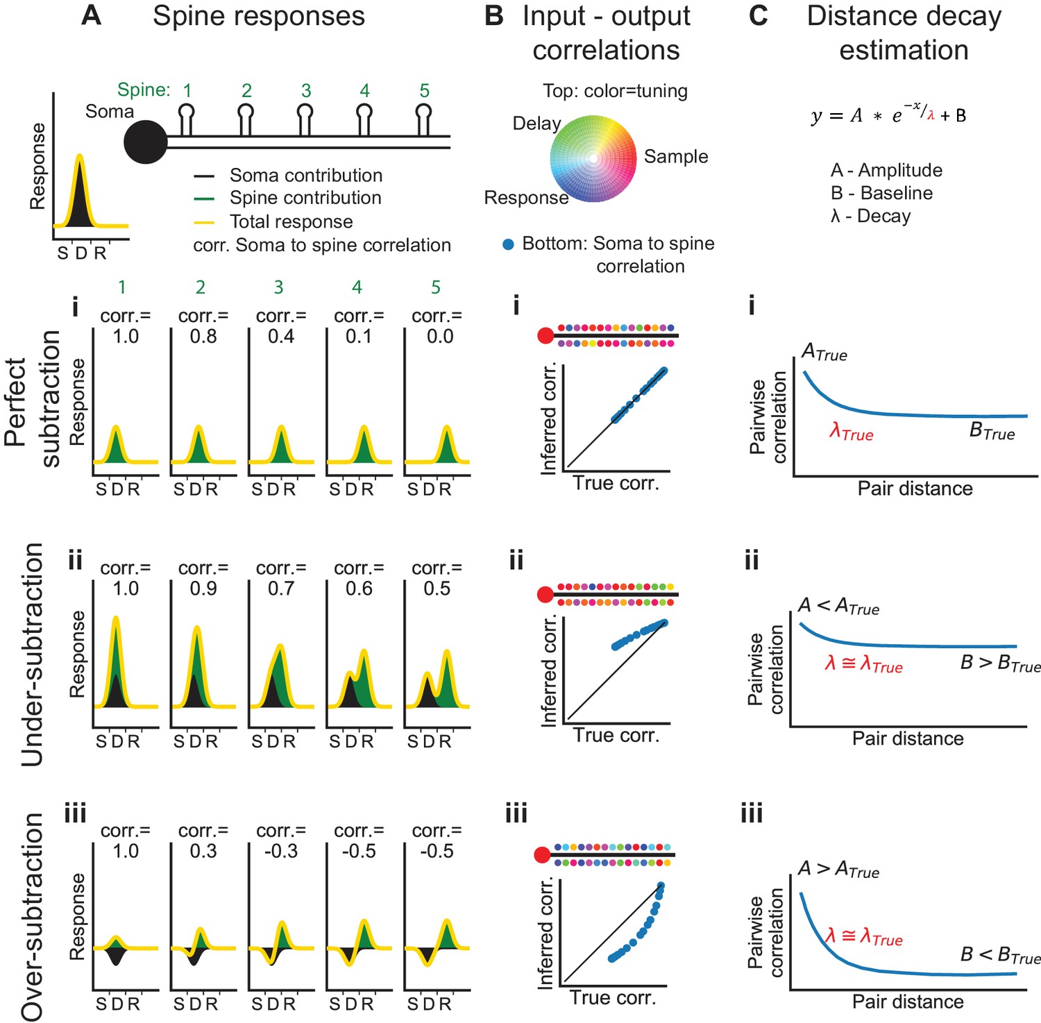
(A) Spine responses under different bAP subtraction regimes. Top, Cartoon of the soma and spatial organization of five spines. Soma trial-average response (black curve) is centered between the sample and delay epochs. (i) True (perfect bAP-component removal) tuning curves for the spines exhibiting a distance-dependent similarity of selectivity. (ii) If the bAP-component is under subtracted, subtracted tuning curves will still be biased towards the somatic selectivity. (iii) If the bAP-component is over subtracted, subtracted tuning curves will be biased away from the somatic selectivity. (B) Input-output correlation under different bAP subtraction regimes. Top, polar RGB representation of spine selectivity as in Figure 5B. (i) With perfect subtraction, the inferred correlation of each spine tuning curve with the somatic tuning curve matches the true correlation (plot). In this cartoon, spine selectivity is biased towards the selectivity of the soma (redder), but there is still significant diversity (green and blue spines). (ii) Under-subtraction of the bAP-component leads to less diverse spine selectivity and higher correlations with the somatic output. (iii) Over-subtraction of the bAP-component leads to more diverse spine selectivity and less correlation with the somatic output than truth. (C) Distance-dependent correlation between pairs of spines can be fit with a three-parameter exponential function. A: magnitude of distance-dependent correlations, λ: length constant, B: magnitude of distance-independent correlations. (i-iii) Different levels of subtraction dramatically shift the inferred values of A and B, but λ is accurately estimated. See also Figure 6—figure supplement 1 for performance of input-output simulation and Figure 6—figure supplement 2 for length constant simulations.
Figure 6—figure supplement 1
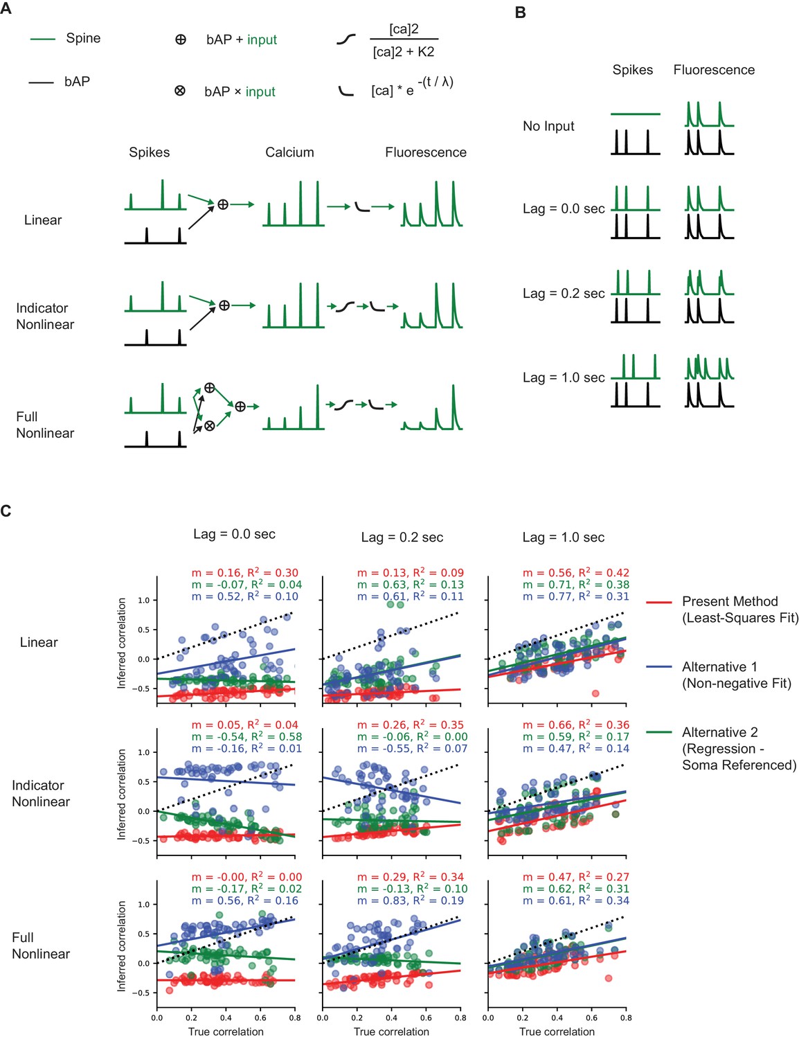
Simulating the effects of removing the estimated bAP-component on the inferred correlation between spines and the reference signal.
(A) Conceptual diagram of three processes for simulating fluorescence at spines from pre- and post-synaptic spiking. Traces are normalized to maximum. (B) Illustration of how the temporal structure of spike correlations influences the discriminability of pre- versus post-synaptic events (linear simulation process shown here). Complete absence of pre-synaptic activity (top row) and perfect correlation of pre- and post-synaptic activity (second row) produce identical normalized fluorescence traces if the correlation is at lag of 0. As lag approaches the decay time constant of the indicator (third row) pre- and post-synaptic transients become more discernable. When lag is far greater than the decay time constant of the indicator transients are easily discriminated in the absence of noise. (C) Inferred correlation between pre-synaptic input and somatic output versus true correlation for three linear subtraction methods (see Materials and methods). Note that for correlations less than or equal to the indicator decay time constant (mean across spines: 200 ms) none of the subtraction methods provides an estimate of input-output correlation that is robustly related to the true correlation (first and second column). Only at lag far greater than decay constant (third column) are inferred correlations informative regardless of simulation process.
Figure 6—figure supplement 2
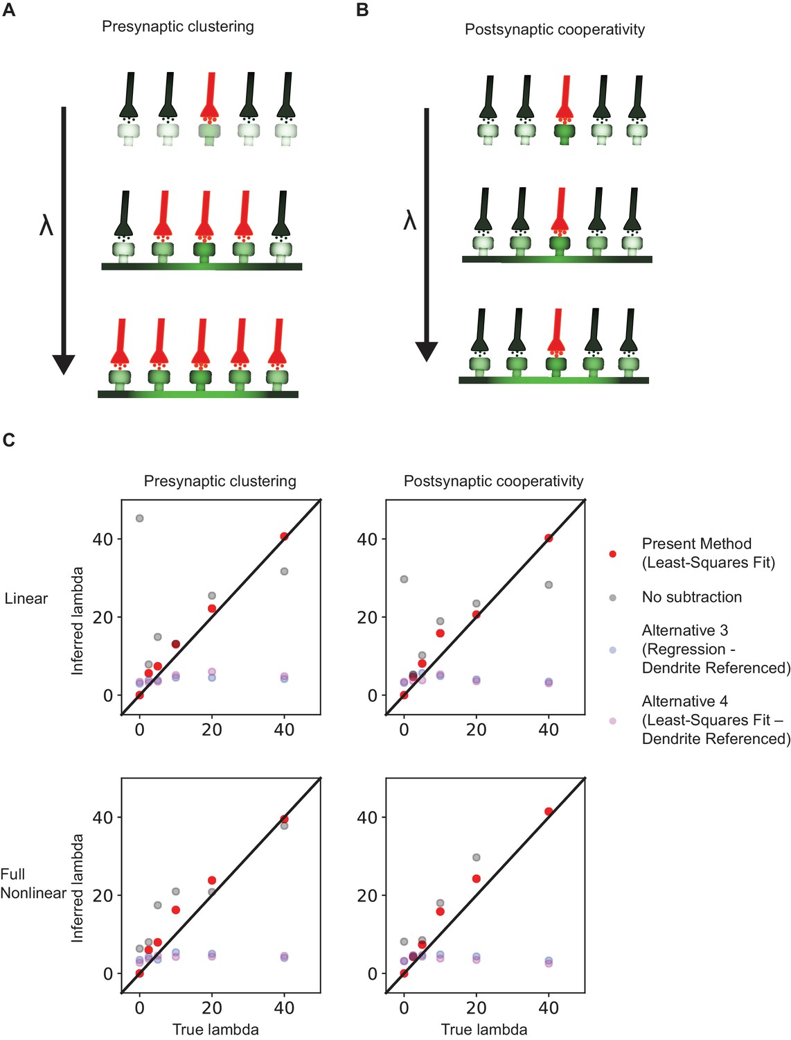
Simulating the effects of removing the estimated bAP-component on the inferred length constant of correlation between spines.
(A) Illustration of simulating pre-synaptic clustering. Correlation in the spiking of pre-synaptic input varied as a function of distance between the inputs along the dendrite. (B) Illustration of simulating post-synaptic cooperativity. Activity at one synapse produces depolarization in neighboring spines (see Materials and methods for details) as a function of distance along the dendrite. (C) Inferred versus true length constant of spine-spine correlation for different simulations and subtraction methods. Length constant = 0 are simulations without clustering or cooperativity. Inferred correlations without significant distance dependence (see Figure 7C) were assigned a length constant of 0. All simulations included distance-dependent variation in decay dynamics. Note that the subtraction method used in this work provides a robust estimate of the length scale (i.e., red points lie near the unity line) regardless of simulation type. Estimates from data without subtraction are less robust (gray points) because distance-dependent decay dynamics (simulated with 30 um spatial scale, see Materials and methods) are not removed. bAP subtraction methods using the nearby dendrite as a reference (blue and magenta points, see Materials and methods) produce uninformative estimates of length constant.
Figure 7
Behavior-related calcium signals are organized in a distance-dependent manner within the dendritic tree.
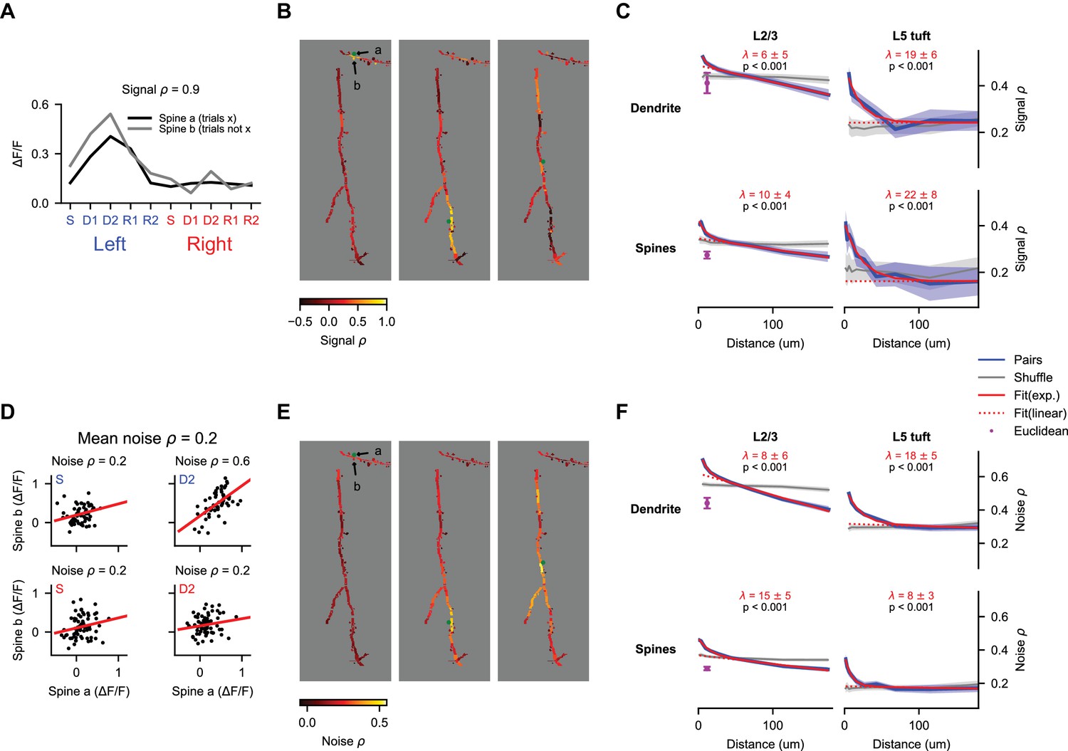
(A) Estimation of pairwise signal correlation after bAP subtraction for two example spines (denoted in (B)). Trial average responses for each epoch and trial type are calculated for each mask from non-overlapping trials (to exclude noise correlations). Signal correlation is the Pearson correlation coefficient between these sets of responses. (B) Pairwise signal correlation of three spines (green dots) with all other masks in an example session (same session as shown in Figure 4C). (C) Pairwise signal correlation as a function of traversal distance through the dendrite (see Materials and methods for binning; L2/3 dendrite: N = 22688 pairs, 1533 segments; L5 dendrite: N = 7468 pairs, 432 segments; L2/3 spines: N = 45993 pairs, 2058 spines; L5 spines: N = 2783 pairs, 285 spines). Shaded regions are ± SEM (see Materials and methods). Magenta point is the mean pairwise correlation of masks with Euclidean distance < 15 μm and traversal distance > 30 μm. Only masks with significant (p < 0.01) task-associated selectivity were included. p-values from nonparametric comparison to shuffle. λ is the mean length constant ± SEM (D) Estimation of pairwise noise correlation for two example spines (denoted in (B)). Each panel is an example epoch denoted by the colored text in the upper left. Each black point is a trial. Noise correlation for a pair is the mean of the correlations calculated across all epochs. (E) Same as (B), but for noise correlation. (F) Same as (C), but for noise correlation. All N same as in (C).
Figure 8
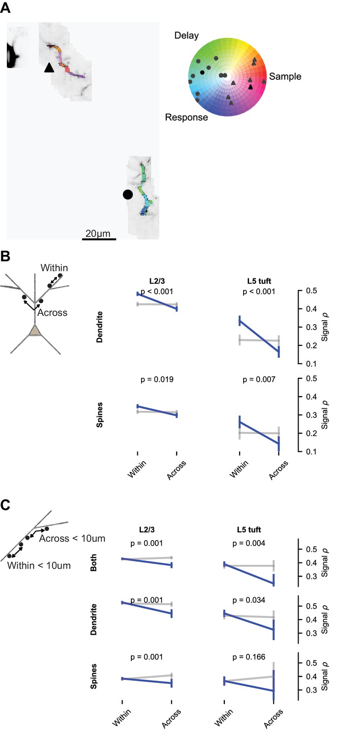
Dendritic branching compartmentalizes behavior-related calcium signals.
(A) Example of clustering of epoch selectivity for a L2/3 session. Hue and saturation were determined for each mask as in Figure 5B after bAP subtraction. Markers (gray: individual masks, black: mean) in the polar plot denote the selectivity of all significantly selective (p<0.01) masks within the branches adjacent to the same marker in the colored MIP. (B) Pairwise signal correlations after bAP subtraction within versus across branches (blue: pairs; gray: shuffle), regardless of distance (L2/3 dendrite within: N = 8794 pairs, 1436 segments; L2/3 dendrite across: N = 13894 pairs, 1403 segments; L5 dendrite within: N = 2652 pairs, 406 segments; L5 dendrite across: N = 4816 pairs, 432 segments; L2/3 spines within: N = 16711 pairs, 2002 spines; L2/3 spines across: N = 29282 pairs, 1907 spines; L5 spines within: N = 1207 pairs, 269 spines; L5 spines across: N = 1576 pairs, 278 spines). (C) Short distance (<10 um) pairwise signal correlations within versus across a branch point (L2/3 both within: N = 10484 pairs, 3510 spines or segments; L2/3 both across: N = 1829 pairs, 814 spines or segments; L5 both within: N = 1368 pairs, 681 spines or segments; L5 both across: N = 139 pairs, 98 spines or segments; L2/3 dendrite within: N = 1533 pairs, 1392 segments; L2/3 dendrite across: N = 359 pairs, 323 segments; L5 dendrite within: N = 451 pairs, 376 segments; L5 dendrite across: N = 61 pairs, 62 segments; L2/3 spines within: N = 3834 pairs, 1929 spines; L2/3 spines across: N = 598 pairs, 400 spines; L5 spines within: N = 228 pairs, 233 spines; L5 spines across: N = 18 pairs, 20 spines). ‘Both’ includes dendrite-dendrite, spine-spine, and spine-dendrite pairs. All plots are mean and SE, p-values from nonparametric permutation test (each spine or dendrite segment drawn only once) comparison to shuffle.
Author response image 1
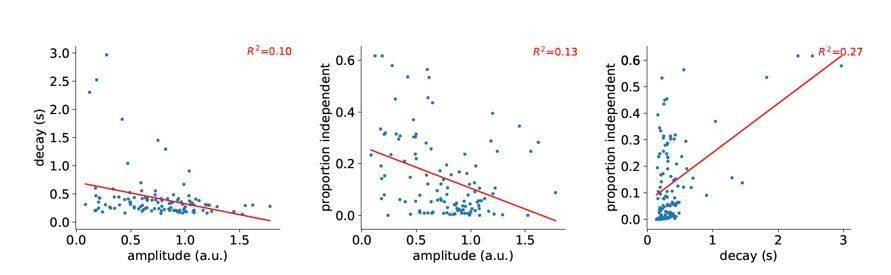
Correlation between decay, amplitude, and proportion independent.
Each point is a 30 μm segment of a L5 tuft dendrite.
Videos
Video 1
Exploring the data online with SpineVis.
In this screencast we show how to use the SpineVis website to look at the data in Figure 2B. On top center is the main viewing area where dragging will change the view in 3D. Clicking on a mask in that window will pull up the fluorescence trace for it in the lower window. The lower window has zoom and pan abilities that are linked to the upper window displaying the timepoint indicated by the black line in the center. To the left are display controls for changing lookup table values and opacity, followed by a timepoint selection window. To the right is the mask lookup window. Below the florescence trace are markers indicating behavioral events (e.g., blue triangle is a lick right event).
Tables
Table 1
SpineVis online viewer links.
Key resources table
| Reagent type (species) or resource | Designation | Source or reference | Identifiers | Additional information |
|---|---|---|---|---|
| Genetic reagent (M. musculus) | Syt17 NO14 (Mouse) | GENSAT | MMRRC Cat# 034355-UCD, RRID: MMRRC_034355-UCD | |
| Genetic reagent (M. musculus) | CamK2a-tTA | JAX | IMSR Cat# JAX:007004, RRID: IMSR_JAX:007004 | |
| Genetic reagent (M. musculus) | Ai93 | JAX | IMSR Cat# JAX:024103, RRID: IMSR_JAX:024103 | |
| Genetic reagent (M. musculus) | Chrna2 OE25 | GENSAT | MMRRC Cat# 036502-UCD, RRID: MMRRC_036502-UCD | |
| Genetic reagent (M. musculus) | ZtTA | JAX | IMSR Cat# JAX: 012266, RRID: IMSR_JAX:012266 | |
| Software and Algorithms | Matlab | Mathworks | RRID:SCR_001622 | |
| Software and Algorithms | ScanImage | Vidrio | RRID:SCR_014307 | |
| Software and Algorithms | Neuromantic | University of Reading | RRID:SCR_013597 | |
| Software and Algorithms | Thunder | Janelia | RRID: SCR_016556 | |
| Software and Algorithms | Spark | Apache | RRID: SCR_016557 | |
| Other | MIMMS microscope 1.0 (2016) | Janelia | RRID:SCR_016511 | |
| Other | Tip-Tilt-Z Sample Positioner | Janelia | RRID:SCR_016528 |
Additional files
Download links
A two-part list of links to download the article, or parts of the article, in various formats.
Downloads (link to download the article as PDF)
Open citations (links to open the citations from this article in various online reference manager services)
Cite this article (links to download the citations from this article in formats compatible with various reference manager tools)
Functional clustering of dendritic activity during decision-making
eLife 8:e46966.
https://doi.org/10.7554/eLife.46966


